如果你也在 怎样代写金融数学Financial Mathematics这个学科遇到相关的难题,请随时右上角联系我们的24/7代写客服。
金融数学是将数学方法应用于金融问题。(有时使用的同等名称是定量金融、金融工程、数学金融和计算金融)。它借鉴了概率、统计、随机过程和经济理论的工具。传统上,投资银行、商业银行、对冲基金、保险公司、公司财务部和监管机构将金融数学的方法应用于诸如衍生证券估值、投资组合结构、风险管理和情景模拟等问题。依赖商品的行业(如能源、制造业)也使用金融数学。 定量分析为金融市场和投资过程带来了效率和严谨性,在监管方面也变得越来越重要。
statistics-lab™ 为您的留学生涯保驾护航 在代写金融数学Financial Mathematics方面已经树立了自己的口碑, 保证靠谱, 高质且原创的统计Statistics代写服务。我们的专家在代写金融数学Financial Mathematics代写方面经验极为丰富,各种代写金融数学Financial Mathematics相关的作业也就用不着说。
我们提供的金融数学Financial Mathematics及其相关学科的代写,服务范围广, 其中包括但不限于:
- Statistical Inference 统计推断
- Statistical Computing 统计计算
- Advanced Probability Theory 高等概率论
- Advanced Mathematical Statistics 高等数理统计学
- (Generalized) Linear Models 广义线性模型
- Statistical Machine Learning 统计机器学习
- Longitudinal Data Analysis 纵向数据分析
- Foundations of Data Science 数据科学基础
金融代写|金融数学代写Financial Mathematics代考|Trajectories of the random walk
Let us begin by defining the simple symmetric random walk.
DEFINITION 3.1.-A simple symmetric random walk on $\mathbb{Z}$ is a sequence $\left(S_{n}\right){n \in \mathbb{N}}$ of random variables such that $-S{0}=x \in \mathbb{Z}$ is deterministic;
$-S_{n+1}=S_{n}+X_{n+1}$ for any $n \in \mathbb{N}$,
where $\left(X_{n}\right){n \geq 1}$ is a sequence of independent random variables with the same Rademache distribution with parameter $1 / 2$ : $$ \mathbb{P}\left(X{1}=-1\right)=\mathbb{P}\left(X_{1}-1\right)=\frac{1}{2} .
$$
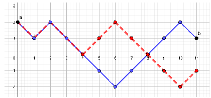
We use the term walk because this process may represent the position of a person who moves in a straight line, with steps of unit length and equal probability of moving forward $(+1)$ or backwards $(-1)$. This walk is said to be simple as we only take steps with amplitude 1 and is said to be symmetric as each increment can be $+1$ or $-1$, with equal probability.
This process may also be used to model the wealth of a gambler who tosses for heads or tails with a balanced coin. Starting from an initial fortune of $S_{0}=x>0$, with each time step, the gambler looses or gains $1 €$ depending on the toss. The variables $X_{n}$ thus represent the gain at the $n$-th game, and $S_{n}$ is the total fortune of the gambler after the $n$-th toss.
Based on this definition, we can easily arrive at the average behavior of the walk.
PROPOSITION 3.1.- For any $n \in \mathbb{N}$, we have
$$
\mathbb{E}\left[S_{n}\right]=S_{0}, \quad \operatorname{Var}\left(S_{n}\right)=n .
$$
PROOF.- Let us first note that
$$
\begin{gathered}
\mathbb{E}\left[X_{1}\right]=(-1) \times \frac{1}{2}+1 \times \frac{1}{2}=0 \
\operatorname{Var}\left(X_{1}\right)=\mathbb{E}\left[X_{1}^{2}\right]=(-1)^{2} \times \frac{1}{2}+1^{2} \times \frac{1}{2}=1
\end{gathered}
$$
the increments are thus centered and reduced. By the linearity of expectation, we obtain
$$
\mathbb{E}\left[S_{n}\right]=\mathbb{E}\left[S_{0}+\sum_{k=1}^{n} X_{k}\right]=S_{0}+\sum_{k=1}^{n} \mathbb{E}\left[X_{k}\right]=S_{0}
$$
since $S_{0}$ is deterministic. Finally, using the independence of the $X_{k}$, we obtain
$$
\operatorname{Var}\left(S_{n}\right)=\operatorname{Var}\left(S_{0}+\sum_{k=1}^{n} X_{k}\right)=\sum_{k=1}^{n} \operatorname{Var}\left(X_{k}\right)=n
$$
hence, the result.
Thus, the walk remains constant on average, but its variance becomes greater over time.
金融代写|金融数学代写Financial Mathematics代考|Reflection principle
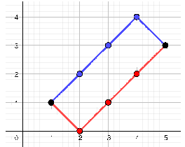
This function defines a bijection between the two sets of paths. Indeed, if we now take a path $\left(\widetilde{S}{m}, \ldots, \widetilde{S}{n}\right)$ from $(m, a)$ to $(n,-b)$, as it takes steps whose amplitude is 1 , since $a>0$ and $-b<0$, this path must necessarily pass through 0 . Let $p$ be the first instant where the path is at 0 . We then construct a path $\left(S_{m}, \ldots, S_{n}\right)$ from $(m, a)$ to $(n, b)$ passing through 0 writing
$$
S_{k}= \begin{cases}\widetilde{S}{k} & \text { if } m \leq k \leq p, \ -\widetilde{S}{k} & \text { if } p \leq k \leq n .\end{cases}
$$
There are, thus, the same number of paths of both types.
An initial application of this property is the following result, called the ballot theorem.
THEOREM 3.1.-During an election with two opposing candidates, $A$ and $B$, candidate $A$ has obtained a votes and candidate $B$ b votes, with $a>b .$ Thus, the probability that $A$ has obtained the majority (in the broad sense) throughout the counting is
$$
p=1-\frac{b}{a+1} .
$$
PROOF.- With all the counts being equiprobable, $p$ is obtained as the ratio of the number of counts with $A$ in the lead all the time to that of the total number of counts. A count can be modeled by a random walk $\left(S_{n}\right)$, where $S_{n}$ is the number of votes by which $A$ is ahead of $B$ after counting the $n$-th ballot.
There are $a+b$ ballots in total and ultimately, $A$ has a lead of $a-b$ votes over $B$; thus, the total number of counts is the number of paths from $(0,0)$ to $(a+b, a-b)$ and has the value $C_{a+b}^{a}$.
The number of counts with $A$ in the lead all long corresponds to
- the number of paths from $(0,0)$ to $(a+b, a-b)$, not taking any strictly negative value; in other words, the number of paths from $(0,0)$ to $(a+b, a-b)$ that do not touch $-1$;
- the number of paths from $(0,1)$ to $(a+b, a-b+1)$ not touching 0 , by shifting the ordinates upwards by one unit;
- the total number of paths from $(0,1)$ to $(a+b, a-b+1)$ minus the number of paths from $(0,1)$ to $(a+b, a-b+1)$ touching 0 ;
- the total number of paths from $(0,1)$ to $(a+b, a-b+1)$ minus the number of paths from $(0,1)$ to $(a+b,-(a-b+1))$ by the reflection principle.
金融代写|金融数学代写Financial Mathematics代考|First return to 0
It is now assumed that the walk starts from $0: S_{0}=0$ and we wish to know whether the walk will return to 0 almost surely. Let us start by observing that if $S_{n}=0$, then $n$ is necessarily even.
PROPOSITION 3.9. – For any $n \in \mathbb{N}$, we have
$$
\mathbb{P}\left(S_{2 n}=0\right)=\frac{1}{4^{n}} C_{2 n^{*}}^{n}
$$
ProOF.- This probability corresponds to the number of paths from $(0,0)$ to $(2 n, 0)$ divided by the total number of paths with length $2 n$, since all the paths are equiprobable. We thus directly have $\mathbb{P}\left(S_{2 n}=0\right)=\frac{C_{2 n}^{n}}{4^{n}}$.
We now look at the first instant of the return to 0 . It is denoted by $T_{0}$. It is, therefore, the random variable
$$
T_{0}=\inf \left{n \geq 1 ; S_{n}=0\right},
$$
using the convention that $\inf \emptyset=+\infty$. It is, therefore, a discrete random variable taking values in $\mathbb{N}^{} \cup{+\infty}$. The distribution of $T_{0}$ can be explicitly calculated. PROPOSITION 3.10.- For any $n \in \mathbb{N}^{}$, we have
$$
\mathbb{P}\left(T_{0}=2 n\right)=\frac{(2 n-2) !}{2^{2 n-1} n !(n-1) !}
$$
ProOF.- The event $\left(T_{0}=2 n\right)$ corresponds to $\left(S_{2} \neq 0, \ldots, S_{2 n-2} \neq 0, S_{2 n}=0\right)$ because then $2 n$ is the first time the walk returns to 0 . In particular, between the instant 0 and the instant $2 n$, the walk does not change in sign and retains the same sign as $S_{1}$. Therefore, we have
$$
\begin{aligned}
\mathbb{P}\left(T_{0}=2 n\right)=& \mathbb{P}\left(S_{1}=1, S_{2}>0, \ldots, S_{2 n-2}>0, S_{2 n}=0\right) \
&+\mathbb{P}\left(S_{1}=-1, S_{2}<0, \ldots, S_{2 n-2}<0, S_{2 n}=0\right) \end{aligned} $$ These two probabilities are equal by symmetry. Further, if $S_{2 n-2}>0$ and $S_{2 n}=0$, then we necessarily have $S_{2 n-1}=1$. Therefore, it follows
$$
\begin{aligned}
\mathbb{P}\left(T_{0}=2 n\right) \
=& 2 \mathbb{P}\left(S_{1}=1, S_{2}>0, \ldots, S_{2 n-2}>0, S_{2 n-1}=1, S_{2 n}=0\right) \
=& 2 \mathbb{P}\left(S_{2 n}=0 \mid S_{1}=1, S_{2}>0, \ldots, S_{2 n-2}>0, S_{2 n-1}=1\right) \
& \times \mathbb{P}\left(S_{1}=1, S_{2}>0, \ldots, S_{2 n-2}>0, S_{2 n-1}=1\right)
\end{aligned}
$$
$$
\begin{aligned}
&=2 \mathbb{P}\left(S_{2 n}=0 \mid S_{2 n-1}=1\right) \mathbb{P}\left(S_{1}=1, S_{2}>0, \ldots, S_{2 n-2}>0, S_{2 n-1}=1\right) \
&=2 \mathbb{P}\left(S_{1}=-1 \mid S_{0}=0\right) \mathbb{P}\left(S_{1}=1, S_{2}>0, \ldots, S_{2 n-2}>0, S_{2 n-1}=1\right) \
&=\mathbb{P}\left(S_{1}=1, S_{2}>0, \ldots, S_{2 n-2}>0, S_{2 n-1}=1\right)
\end{aligned}
$$
using the Markov property, the stationary property and then the fact that
$$
\mathbb{P}\left(S_{1}=-1 \mid S_{0}=0\right)=\mathbb{P}\left(S_{1}=-1\right)=\mathbb{P}\left(X_{1}=-1\right)=\frac{1}{2}
$$
金融数学代考
金融代写|金融数学代写Financial Mathematics代考|Trajectories of the random walk
让我们从定义简单的对称随机游走开始。
定义 3.1.-一个简单的对称随机游走从是一个序列(小号n)n∈ñ随机变量,使得−小号0=X∈从是确定性的;
−小号n+1=小号n+Xn+1对于任何n∈ñ,
其中(Xn)n≥1是一系列独立随机变量,具有相同的 Rademache 分布和参数1/2 :
磷(X1=−1)=磷(X1−1)=12.
我们使用术语 walk 是因为这个过程可能代表一个人在直线上移动的位置,具有单位长度的步长和相同的前进概率(+1)或向后(−1). 据说这种步行很简单,因为我们只采取幅度为 1 的步骤,并且据说是对称的,因为每个增量都可以是+1或者−1,等概率。
这个过程也可以用来模拟一个赌徒的财富,他用平衡的硬币投掷正面或反面。从最初的财富开始小号0=X>0, 每一个时间步,赌徒输或赢€1€取决于折腾。变量Xn因此代表在n-th 游戏,和小号n是赌徒之后的总财富n-th 折腾。
基于这个定义,我们可以很容易地得出步行的平均行为。
提案 3.1.- 对于任何n∈ñ, 我们有
和[小号n]=小号0,曾是(小号n)=n.
证明-让我们首先注意到
和[X1]=(−1)×12+1×12=0 曾是(X1)=和[X12]=(−1)2×12+12×12=1
增量因此被集中和减少。通过期望的线性,我们得到
和[小号n]=和[小号0+∑ķ=1nXķ]=小号0+∑ķ=1n和[Xķ]=小号0
自从小号0是确定性的。最后,利用独立性Xķ, 我们获得
曾是(小号n)=曾是(小号0+∑ķ=1nXķ)=∑ķ=1n曾是(Xķ)=n
因此,结果。
因此,平均而言,步行保持不变,但随着时间的推移,其方差会变得更大。
金融代写|金融数学代写Financial Mathematics代考|Reflection principle
该函数定义了两组路径之间的双射。的确,如果我们现在走一条路(小号~米,…,小号~n)从(米,一个)至(n,−b), 因为它采取幅度为 1 的步骤, 因为一个>0和−b<0,这条路径必然经过 0 。让p成为路径位于 0 的第一个时刻。然后我们构造一条路径(小号米,…,小号n)从(米,一个)至(n,b)通过0写
小号ķ={小号~ķ 如果 米≤ķ≤p, −小号~ķ 如果 p≤ķ≤n.
因此,两种类型的路径数量相同。
该属性的初始应用是以下结果,称为投票定理。
定理 3.1.-在有两个反对候选人的选举中,一个和乙, 候选人一个获得了选票和候选人乙b 票,与一个>b.因此,概率一个在整个计数过程中获得多数(广义上)是
p=1−b一个+1.
证明-所有计数都是等概率的,p获得为计数的数量与一个一直领先于总计数。计数可以通过随机游走来建模(小号n), 在哪里小号n是投票数一个领先于乙数完之后n-th 选票。
有一个+b总票数和最终票数,一个领先于一个−b投票通过乙; 因此,计数的总数是从(0,0)至(一个+b,一个−b)并且有价值C一个+b一个.
计数与一个在领先的所有长对应
- 从路径数(0,0)至(一个+b,一个−b),不取任何严格的负值;换句话说,从(0,0)至(一个+b,一个−b)不接触的−1;
- 从路径数(0,1)至(一个+b,一个−b+1)不接触 0 ,将纵坐标向上移动一个单位;
- 路径总数(0,1)至(一个+b,一个−b+1)减去从(0,1)至(一个+b,一个−b+1)触摸 0 ;
- 路径总数(0,1)至(一个+b,一个−b+1)减去从(0,1)至(一个+b,−(一个−b+1))通过反射原理。
金融代写|金融数学代写Financial Mathematics代考|First return to 0
现在假设步行从0:小号0=0我们想知道步行是否几乎肯定会回到 0。让我们首先观察如果小号n=0, 然后n必然是偶数。
提案 3.9。– 对于任何n∈ñ, 我们有
磷(小号2n=0)=14nC2n∗n
ProOF.- 这个概率对应于从(0,0)至(2n,0)除以有长度的路径总数2n,因为所有路径都是等概率的。因此我们直接有磷(小号2n=0)=C2nn4n.
我们现在看看返回 0 的第一时刻。它表示为吨0. 因此,它是随机变量
T_{0}=\inf \left{n \geq 1 ; S_{n}=0\right},T_{0}=\inf \left{n \geq 1 ; S_{n}=0\right},
使用约定信息∅=+∞. 因此,它是一个离散随机变量,取值ñ∪+∞. 的分布吨0可以显式计算。提案 3.10.- 对于任何n∈ñ, 我们有
磷(吨0=2n)=(2n−2)!22n−1n!(n−1)!
证明.- 事件(吨0=2n)对应于(小号2≠0,…,小号2n−2≠0,小号2n=0)因为那时2n是第一次步行返回 0 。特别是在时刻 0 和时刻之间2n, walk 的符号不变并保持与小号1. 因此,我们有
磷(吨0=2n)=磷(小号1=1,小号2>0,…,小号2n−2>0,小号2n=0) +磷(小号1=−1,小号2<0,…,小号2n−2<0,小号2n=0)这两个概率是对称的。此外,如果小号2n−2>0和小号2n=0,那么我们必然有小号2n−1=1. 因此,它遵循
磷(吨0=2n) =2磷(小号1=1,小号2>0,…,小号2n−2>0,小号2n−1=1,小号2n=0) =2磷(小号2n=0∣小号1=1,小号2>0,…,小号2n−2>0,小号2n−1=1) ×磷(小号1=1,小号2>0,…,小号2n−2>0,小号2n−1=1)
=2磷(小号2n=0∣小号2n−1=1)磷(小号1=1,小号2>0,…,小号2n−2>0,小号2n−1=1) =2磷(小号1=−1∣小号0=0)磷(小号1=1,小号2>0,…,小号2n−2>0,小号2n−1=1) =磷(小号1=1,小号2>0,…,小号2n−2>0,小号2n−1=1)
使用马尔可夫性质,平稳性质,然后是
磷(小号1=−1∣小号0=0)=磷(小号1=−1)=磷(X1=−1)=12

统计代写请认准statistics-lab™. statistics-lab™为您的留学生涯保驾护航。
金融工程代写
金融工程是使用数学技术来解决金融问题。金融工程使用计算机科学、统计学、经济学和应用数学领域的工具和知识来解决当前的金融问题,以及设计新的和创新的金融产品。
非参数统计代写
非参数统计指的是一种统计方法,其中不假设数据来自于由少数参数决定的规定模型;这种模型的例子包括正态分布模型和线性回归模型。
广义线性模型代考
广义线性模型(GLM)归属统计学领域,是一种应用灵活的线性回归模型。该模型允许因变量的偏差分布有除了正态分布之外的其它分布。
术语 广义线性模型(GLM)通常是指给定连续和/或分类预测因素的连续响应变量的常规线性回归模型。它包括多元线性回归,以及方差分析和方差分析(仅含固定效应)。
有限元方法代写
有限元方法(FEM)是一种流行的方法,用于数值解决工程和数学建模中出现的微分方程。典型的问题领域包括结构分析、传热、流体流动、质量运输和电磁势等传统领域。
有限元是一种通用的数值方法,用于解决两个或三个空间变量的偏微分方程(即一些边界值问题)。为了解决一个问题,有限元将一个大系统细分为更小、更简单的部分,称为有限元。这是通过在空间维度上的特定空间离散化来实现的,它是通过构建对象的网格来实现的:用于求解的数值域,它有有限数量的点。边界值问题的有限元方法表述最终导致一个代数方程组。该方法在域上对未知函数进行逼近。[1] 然后将模拟这些有限元的简单方程组合成一个更大的方程系统,以模拟整个问题。然后,有限元通过变化微积分使相关的误差函数最小化来逼近一个解决方案。
tatistics-lab作为专业的留学生服务机构,多年来已为美国、英国、加拿大、澳洲等留学热门地的学生提供专业的学术服务,包括但不限于Essay代写,Assignment代写,Dissertation代写,Report代写,小组作业代写,Proposal代写,Paper代写,Presentation代写,计算机作业代写,论文修改和润色,网课代做,exam代考等等。写作范围涵盖高中,本科,研究生等海外留学全阶段,辐射金融,经济学,会计学,审计学,管理学等全球99%专业科目。写作团队既有专业英语母语作者,也有海外名校硕博留学生,每位写作老师都拥有过硬的语言能力,专业的学科背景和学术写作经验。我们承诺100%原创,100%专业,100%准时,100%满意。
随机分析代写
随机微积分是数学的一个分支,对随机过程进行操作。它允许为随机过程的积分定义一个关于随机过程的一致的积分理论。这个领域是由日本数学家伊藤清在第二次世界大战期间创建并开始的。
时间序列分析代写
随机过程,是依赖于参数的一组随机变量的全体,参数通常是时间。 随机变量是随机现象的数量表现,其时间序列是一组按照时间发生先后顺序进行排列的数据点序列。通常一组时间序列的时间间隔为一恒定值(如1秒,5分钟,12小时,7天,1年),因此时间序列可以作为离散时间数据进行分析处理。研究时间序列数据的意义在于现实中,往往需要研究某个事物其随时间发展变化的规律。这就需要通过研究该事物过去发展的历史记录,以得到其自身发展的规律。
回归分析代写
多元回归分析渐进(Multiple Regression Analysis Asymptotics)属于计量经济学领域,主要是一种数学上的统计分析方法,可以分析复杂情况下各影响因素的数学关系,在自然科学、社会和经济学等多个领域内应用广泛。
MATLAB代写
MATLAB 是一种用于技术计算的高性能语言。它将计算、可视化和编程集成在一个易于使用的环境中,其中问题和解决方案以熟悉的数学符号表示。典型用途包括:数学和计算算法开发建模、仿真和原型制作数据分析、探索和可视化科学和工程图形应用程序开发,包括图形用户界面构建MATLAB 是一个交互式系统,其基本数据元素是一个不需要维度的数组。这使您可以解决许多技术计算问题,尤其是那些具有矩阵和向量公式的问题,而只需用 C 或 Fortran 等标量非交互式语言编写程序所需的时间的一小部分。MATLAB 名称代表矩阵实验室。MATLAB 最初的编写目的是提供对由 LINPACK 和 EISPACK 项目开发的矩阵软件的轻松访问,这两个项目共同代表了矩阵计算软件的最新技术。MATLAB 经过多年的发展,得到了许多用户的投入。在大学环境中,它是数学、工程和科学入门和高级课程的标准教学工具。在工业领域,MATLAB 是高效研究、开发和分析的首选工具。MATLAB 具有一系列称为工具箱的特定于应用程序的解决方案。对于大多数 MATLAB 用户来说非常重要,工具箱允许您学习和应用专业技术。工具箱是 MATLAB 函数(M 文件)的综合集合,可扩展 MATLAB 环境以解决特定类别的问题。可用工具箱的领域包括信号处理、控制系统、神经网络、模糊逻辑、小波、仿真等。