如果你也在 怎样代写金融数学Financial Mathematics这个学科遇到相关的难题，请随时右上角联系我们的24/7代写客服。

金融数学是将数学方法应用于金融问题。(有时使用的同等名称是定量金融、金融工程、数学金融和计算金融）。它借鉴了概率、统计、随机过程和经济理论的工具。传统上，投资银行、商业银行、对冲基金、保险公司、公司财务部和监管机构将金融数学的方法应用于诸如衍生证券估值、投资组合结构、风险管理和情景模拟等问题。依赖商品的行业（如能源、制造业）也使用金融数学。 定量分析为金融市场和投资过程带来了效率和严谨性，在监管方面也变得越来越重要。

statistics-lab™ 为您的留学生涯保驾护航 在代写金融数学Financial Mathematics方面已经树立了自己的口碑, 保证靠谱, 高质且原创的统计Statistics代写服务。我们的专家在代写金融数学Financial Mathematics代写方面经验极为丰富，各种代写金融数学Financial Mathematics相关的作业也就用不着说。

我们提供的金融数学Financial Mathematics及其相关学科的代写，服务范围广, 其中包括但不限于:

• Statistical Inference 统计推断
• Statistical Computing 统计计算
• Advanced Probability Theory 高等概率论
• Advanced Mathematical Statistics 高等数理统计学
• (Generalized) Linear Models 广义线性模型
• Statistical Machine Learning 统计机器学习
• Longitudinal Data Analysis 纵向数据分析
• Foundations of Data Science 数据科学基础

金融代写|金融数学作业代写Financial Mathematics代考|Valuation of Credit Default Swaps

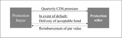
Hull and White (2001) focus on CDSs with periodical risk-free premium payments in arrear. Moreover, the protection buyer is regarded as a risk-free agent and therefore the payments of the buyer are risk-free as well.
The following swap payment streams are considered for our analysis:

1. Risk seller $A$ pays the swap rate till maturity $T$. If the first default occurs before $T$ then A terminates his regular payments and
   a. pays a final accrual payment ${ }^{*}$ of $e$, if the defaulted party is the reference obligator $R$, otherwise
   b. pays no final accrual payment, if the risk buyer $B$ defaults.
2. If $R$ defaults during the duration of the swap and before $B$, then $B$ pays the difference between the face value of the debt claim of $A$ against $R$ and the recovery rate. The recovery rate is calculated as the face value of the bond including accrued interests.
3. If $B$ defaults before $R$ during the duration, then no payment will be made and the swap is going to be terminated.
   At $t=0$ the present value of the expected premium paid by $A$ is calculated as follows:
   $$
   \dddot{\kappa}{\rho v}^{\prime}=\dddot{\kappa}^{\prime}\left(\int{0}^{T}\left{f_{t}^{R B}\left[u_{t}+m_{t}\left(e w^{-1}\right)\right]+f_{t}^{\mathrm{BR}} u_{t}\right} \mathrm{d} t+G_{T}^{\mathrm{BR}} u_{T}\right)
   $$
   where, $w$ represents the annual payments of the premium calculated as a proportion of the face value of the swaps, $f_{t}^{R B}$ is the default density of $R$ under the condition that $B$ did not default until $t=0,{ }^{\dagger} f_{t}^{\mathrm{B} R}$ stands for the default density function of $B$ under the assumption that $R$ do not default until $t=0, \mp u_{t}$ represents the present value of the annuity factor for annuity payments of 1 within the period $[0 ; t], m_{t}\left(e^{-1}\right)$ describes the present value factor of an one-off final payment of $e w^{-1}$ in $t$, and $G_{T}^{\mathrm{BR}}$ is the probability that the counterparty $B$ and the reference entity $R$ do not default until $T$.

The value of the swap for $A$ is calculated as the present value of the expected payments generated by the swap as follows:
$$
\ddot{\varpi}{0}^{\prime}=\int{0}^{T}\left[1-E\left(\delta_{t}^{R}\right)\left(1+c_{t}\right)\right] f_{t}^{R B} m_{t}(1) \mathrm{d} t
$$

where $\delta_{t}^{R}$ is the expected recovery rate at the default of $R$ and $c_{t}$ represents the interest accruals until $t$ is calculated as a percentage of the face value on the debt claims.

Hull and White (2001) calculate the fair swap-rate $\dddot{\kappa}{\rho \nu}^{\prime}$ drawing on Equations $2.2$ and $2.3$ through using a Monte Carlo simulation. They use different sets of parameters first for the quality of the risk buyer and second for the correlation between the risk buyer and the reference entity. This fair swap rate equals $w$, from which it follows that $\ddot{\varpi}{0}^{\prime}=\dddot{\kappa}_{\rho v^{\prime}}$ High correlations between the risk buyer and the reference entity as well as low ratings of the swap seller show a significant impact on the swap rate.

金融代写|金融数学作业代写Financial Mathematics代考|Assumptions

To evaluate vulnerable puts, different methods (e.g., Johnson and Stulz 1987, Klein 1996, Klein and Inglis 1999) based on Merton’s (1974) credit risk model have been proposed. ${ }^{\dagger}$ Looking at defaultable CDSs, both credit risks have to be considered explicitly: First, the credit risk of the reference asset and second the credit risk of the risk buyer have to be evaluated. It should be noted that the valuation of these credit risks does not have to be based on an identical methodology. For the purpose of this review chapter, we assume a standard Merton (1974) firm value model:

• Firm value of the risk buyer $V_{t}^{\mathrm{B}}$ follows a lognormal distribution. The process of $V_{t}^{\mathrm{B}}$ can be expressed as follows: $\mathrm{d} V_{t}^{R}=V_{t}^{\mathrm{B}} \mu_{V^{\mathrm{B}}} \mathrm{d} t+V_{t}^{\mathrm{B}} \sigma_{V^{\mathrm{B}}} \mathrm{d} W_{t}^{V^{\mathrm{B}}}$.
• Firm value of the reference party $V_{t}^{R}$ follows a lognormal distribution. We are therefore able to use the following expression:
  $$
  \mathrm{d} V_{t}^{R}=V_{t}^{R} \mu_{V^{R}} \mathrm{~d} t+V_{t}^{R} \sigma_{V^{R}} \mathrm{~d} W_{t}^{V^{\mathbb{R}}}
  $$
  The correlation coefficient between the firm values $B$ and $R$, both of which follow a Brownian motion, is denoted as $\rho_{\mathrm{B} R}$.Risk buyer $B$ defaults only at $T$. The default occurs, if the firm’s value $V_{t}^{\mathrm{B}}$ drops below an assessed fixed default barrier. This threshold level differs, as shown below, between the various models used to evaluate vulnerable puts:
• a. Option (a): The claim of the swap can be used as the default barrier. This is equivalent to the assumption that the default swap is the sole liability of the option writer and therefore this follows Johnson and Stulz (1987).
• b. Option (b): Alternatively, the total amount of all liabilities of the risk buyer can be drawn on as the default barrier. If the liabilities are assumed to be constant over time, then this is equivalent to the assumption that the claim of the swap is negligibly small. This is based on the model of Klein (1996) and Klein and Inglis $(1999) ^{}$
• c. Option (c): Moreover, the threshold level can be set equivalent to the sum of all other liabilities of the option writer additional to the claim on the swap. This is based on the approach of Klein and Inglis (2001).
• Reference party $R$ can only default at $T$. The default occurs, if the firm value $V_{T}^{R}$ drops below the value of the liabilities.
• At default, the recovery rate $\delta_{T}^{\mathrm{B}}\left(V_{T}^{\mathrm{B}}\right)$ of the risk taker $B$ is calculated as the ratio of the firm value $V_{T}^{\mathrm{B}}$ and the total sum of all liabilities multiplied with the factor $(1-\alpha)$. The latter factor represents the dead-weighted costs associated with the default.
• At default, the recovery rate of $R$ corresponds to the ratio of $V_{T}^{R}$ to the overall liabilities.

金融代写|金融数学作业代写Financial Mathematics代考|Valuation of Credit Default Swaps

The value of the CDS, $\ddot{\varpi}{0}$, can be derived from the discounted expected stream of payments. The expected values each depending on the default barrier of $\mathrm{B}$ can be expressed as follows: $$ \begin{aligned} \ddot{\varpi}{0}^{\prime}=& E_{p^{}}\left{B_{T}^{-1}\left[\left(F-V_{T}^{R}\right)^{+} \mathbf{1}{\left{V{T}^{\mathrm{B}} \geq F-V_{T}^{\mathbb{\pi}}\right}}+V_{T}^{\mathrm{B}} \mathbf{1}{\left{V{T}^{\mathrm{B}}{0}^{\prime \prime}=& E{p^{}}\left{B_{T}^{-1}\left[\left(F-V_{T}^{R}\right)^{+} \mathbf{1}{\left{V{T}^{\mathrm{B}} \geq D^{\mathrm{B}}\right}}+(1-\alpha) \frac{V_{T}^{\mathrm{B}}}{D^{}}\left(F-V_{T}^{R}\right)+\mathbf{1}{\left{V{T}^{\mathrm{B}}{0}^{\prime \prime \prime}=& E{p^{}}\left[B_{T}^{-1}\left(\left(F-V_{T}^{R}\right)^{+} \mathbf{1}{\left{V{T}^{\mathrm{B}} \geq D^{\mathrm{B}}+F-V_{T}^{\mathrm{R}}\right.}\right}\right.\
&\left.\left.+(1-\alpha) \frac{V_{T}^{\mathrm{B}}}{D^{}+\left(F-V_{T}^{R}\right)}\left(F-V_{T}^{R}\right)^{+} \mathbf{1}{\left{V{T}^{\mathrm{B}}{0}^{\prime}$ to $\ddot{\varpi}{0}^{\prime \prime \prime}$ represent the above described options (a) to (c), respectively. The CDS equals considering its payout-structure a defaultable put option, which is expressed as $\tilde{P}{0}\left(F, V{t}^{R}\right)$. Owing to this, the equations for European put options derived by Johnson and Stulz (1987), Klein (1996), and Klein and Inglis (2001) can be used to determine the expected rate of return in Equation 2.4. We use $\ddot{\varpi} 0_{0}^{\prime \prime}$ below as illustrative example: $$ \begin{aligned} \ddot{\omega}{t}^{\prime \prime}=&-V{t}^{R} \Phi_{2}\left(-d_{1}, b_{1},-p\right)+F \mathrm{e}^{-r(T-t)} \Phi_{2}\left(-d_{2}, b_{2},-p\right) \ &-(1-\alpha) \frac{V_{t}^{\mathrm{B}}}{D^{\star}} V_{t}^{R} \mathrm{e}^{p \sigma} v^{\mathrm{B}^{\alpha}} v^{R^{(T-t)}} \mathrm{e}^{r(T-t)} \Phi_{2}\left(-\tilde{d}{1}, \tilde{b}{1}, p\right) \ &+(1-\alpha) \frac{V_{t}^{\mathrm{B}}}{D^{\star}} F \Phi_{2}\left(-\tilde{d}{2}, \tilde{b}{2}, p\right) \end{aligned} $$ where $\Phi_{2}(\cdot)$ is the function with a standard bivariate normal distribution and $d_{1}, d_{2}, b_{1}, b_{2}$, $t^{}$, and $p$ are give by:
$d_{1}=\frac{\ln \left(V_{t}^{R} / F\right)+\left(r+\frac{1}{2} \sigma_{V^{R}}^{2}\right) t^{}}{\sigma_{V^{\mathbb{R}} \sqrt{t^{}}}}=d_{1}\left(t^{}, V_{t}^{R}\right), \quad \tilde{d}{1}=d{1}+p \sigma_{V^{\mathrm{B}}} \sqrt{t^{}}$
$d_{2}=d_{1}-\sigma_{V^{\mathbb{R}} \sqrt{t^{}}} \quad \tilde{d}{2}=d{2}+p \sigma_{V^{\mathrm{B}}} \sqrt{t^{}}$
$b_{1}=\frac{\ln \left(V_{t}^{\mathrm{B}} / D^{}\right)+\left(r-\frac{1}{2} \sigma_{V^{\mathrm{B}}}^{2}+p \sigma_{V^{\mathrm{B}}} \sigma_{V^{\mathrm{R}}}\right) t^{}}{\sigma_{V^{\mathrm{B}}} \sqrt{t^{}}}=b_{1}\left(t^{\star}, V_{t}^{\mathrm{B}}\right), \quad \tilde{b}{1}=-b{1}-\sigma_{V^{\mathrm{B}}} \sqrt{t^{\star}}$
$b_{2}=b_{1}-p \sigma_{V^{\mathbb{n}}} \sqrt{t^{}}$,
$\tilde{b}{2}=-b{2}-\sigma_{V^{\mathrm{B}}} \sqrt{t^{\star}}$
$t^{*}=T-t$
$\rho=\rho_{\mathrm{BR}}$
This equation follows directly from Klein’s (1996) equation for European put options with a defaultable option writer and a constant interest rate. Within this framework, the firm

value $V$ of the option writer, the value of the underlying $U$, and the strike price $K$ are specified as follows:*
$$
\begin{gathered}
V_{t}=V_{t}^{\mathrm{B}} \
U_{t}=V_{t}^{R} \
K=F
\end{gathered}
$$
In the case of stochastic interest rates, the equation framework of Klein and Inglis (1999) has to be used instead of Klein’s framework. ${ }^{\dagger}$

金融数学代写

金融代写|金融数学作业代写Financial Mathematics代考|Valuation of Credit Default Swaps

Hull 和 White (2001) 专注于定期无风险支付拖欠保费的 CDS。此外，保护买方被视为无风险代理人，因此买方的付款也是无风险的。
我们的分析考虑了以下掉期支付流：

1. 风险卖方一种支付掉期利率直到到期吨. 如果第一个默认值发生在之前吨然后 A 终止他的定期付款和
   a。支付最终应计付款∗的和, 如果违约方是参考义务人R, 否则
   b. 如果风险买方不支付最终应计付款乙默认值。
2. 如果R在交换期间和之前的默认值乙， 然后乙支付债权面值的差额一种反对R和恢复率。回收率按包括应计利息在内的债券面值计算。
3. 如果乙之前的默认值R在此期间，将不支付任何款项，并且将终止掉期。
   在吨=0支付的预期保费的现值一种计算如下：
   \dddot{\kappa}{\rho v}^{\prime}=\dddot{\kappa}^{\prime}\left(\int{0}^{T}\left{f_{t}^{R B }\left[u_{t}+m_{t}\left(e w^{-1}\right)\right]+f_{t}^{\mathrm{BR}} u_{t}\right} \mathrm {d} t+G_{T}^{\mathrm{BR}} u_{T}\right)\dddot{\kappa}{\rho v}^{\prime}=\dddot{\kappa}^{\prime}\left(\int{0}^{T}\left{f_{t}^{R B }\left[u_{t}+m_{t}\left(e w^{-1}\right)\right]+f_{t}^{\mathrm{BR}} u_{t}\right} \mathrm {d} t+G_{T}^{\mathrm{BR}} u_{T}\right)
   在哪里，在表示按掉期面值的比例计算的每年支付的保费，F吨R乙是默认密度R条件下乙直到没有违约吨=0,†F吨乙R代表默认的密度函数乙在假设R不要默认，直到吨=0,∓在吨表示该期间内年金支付为 1 的年金因子的现值[0;吨],米吨(和−1)描述一次性最终付款的现值因子和在−1在吨， 和G吨乙R是交易对手的概率乙和参考实体R不要默认，直到吨.

掉期的价值一种计算为掉期产生的预期支付的现值，如下所示：
ϖ¨0′=∫0吨[1−和(d吨R)(1+C吨)]F吨R乙米吨(1)d吨

在哪里d吨R是默认情况下的预期回收率R和C吨表示应计利息，直到吨按债权面值的百分比计算。

Hull and White (2001) 计算公平掉期利率ķ⃛ρν′绘制方程2.2和2.3通过使用蒙特卡罗模拟。他们首先对风险购买者的质量使用不同的参数集，其次对风险购买者和参考实体之间的相关性使用不同的参数集。这个公平的掉期利率等于在，由此得出ϖ¨0′=ķ⃛ρ在′风险买方和参考实体之间的高相关性以及掉期卖方的低评级表明对掉期利率有重大影响。

金融代写|金融数学作业代写Financial Mathematics代考|Assumptions

为了评估易受攻击的看跌期权，基于 Merton (1974) 信用风险模型提出了不同的方法（例如 Johnson 和 Stulz 1987、Klein 1996、Klein 和 Inglis 1999）。†对于可违约 CDS，必须明确考虑两种信用风险：首先，必须评估参考资产的信用风险，其次必须评估风险买方的信用风险。应该注意的是，这些信用风险的估值不必基于相同的方法。出于本章回顾的目的，我们假设一个标准的 Merton (1974) 公司价值模型：

• 风险买方的公司价值在吨乙服从对数正态分布。的过程在吨乙可以表示如下：d在吨R=在吨乙μ在乙d吨+在吨乙σ在乙d在吨在乙.
• 参考方的公司价值在吨R服从对数正态分布。因此，我们可以使用以下表达式：
  d在吨R=在吨Rμ在R d吨+在吨Rσ在R d在吨在R
  公司价值之间的相关系数乙和R，两者都遵循布朗运动，记为ρ乙R.风险买家乙默认仅在吨. 默认发生，如果公司的价值在吨乙跌至评估的固定默认障碍以下。如下所示，用于评估易受攻击看跌期权的各种模型之间的阈值水平不同：
• 一种。选项（a）：可以将交换的声明用作默认障碍。这相当于假设违约掉期是期权卖方的唯一责任，因此遵循 Johnson 和 Stulz (1987)。
• 湾。选项（b）：或者，可以将风险买方的所有负债总额作为违约障碍。如果假设负债随着时间的推移是恒定的，那么这相当于假设掉期的债权可以忽略不计。这是基于 Klein (1996) 和 Klein and Inglis $(1999) ^{ }$的模型
• C。选项（c）：此外，阈值水平可以设置为等于期权卖方除掉期债权之外的所有其他负债的总和。这是基于 Klein 和 Inglis (2001) 的方法。
• 参考方R只能默认为吨. 默认发生，如果坚定的价值在吨R低于负债的价值。
• 默认情况下，恢复率d吨乙(在吨乙)冒险者的乙计算为公司价值的比率在吨乙和所有负债的总和乘以因子(1−一种). 后一个因素代表与违约相关的无谓加权成本。
• 默认情况下，恢复率为R对应的比例在吨R对总负债。

金融代写|金融数学作业代写Financial Mathematics代考|Valuation of Credit Default Swaps

CDS的价值，ϖ¨0, 可以从贴现的预期支付流中推导出来。每个期望值取决于乙可以表示如下： $$ \begin{aligned} \ddot{\varpi}{0}^{\prime}=& E_{p^{}}\left{B_{T}^{-1}\left [\left(F-V_{T}^{R}\right)^{+} \mathbf{1}{\left{V{T}^{\mathrm{B}} \geq F-V_{T} ^{\mathbb{\pi}}\right}}+V_{T}^{\mathrm{B}} \mathbf{1}{\left{V{T}^{\mathrm{B}}{0} ^{\prime \prime}=& E{p^{}}\left{B_{T}^{-1}\left[\left(F-V_{T}^{R}\right)^{+ } \mathbf{1}{\left{V{T}^{\mathrm{B}} \geq D^{\mathrm{B}}\right}}+(1-\alpha) \frac{V_{T }^{\mathrm{B}}}{D^{}}\left(F-V_{T}^{R}\right)+\mathbf{1}{\left{V{T}^{\mathrm {B}}{0}^{\prime \prime \prime}=& E{p^{}}\left[B_{T}^{-1}\left(\left(F-V_{T}^ {R}\right)^{+} \mathbf{1}{\left{V{T}^{\mathrm{B}} \geq D^{\mathrm{B}}+F-V_{T}^ {\mathrm{R}}\right.}\right}\right.\
&\left.\left.+(1-\alpha) \frac{V_{T}^{\mathrm{B}}}{D^{}+\left(F-V_{T}^{R}\右)}\left(F-V_{T}^{R}\right)^{+} \mathbf{1}{\left{V{T}^{\mathrm{B}}{0}^{\主要}吨这\ddot {\varpi} {0} ^ {\素数\素数\素数}r和pr和s和n吨吨H和一种b这在和d和sCr一世b和d这p吨一世这ns(一种)吨这(C),r和sp和C吨一世在和l是.吨H和CD小号和q在一种lsC这ns一世d和r一世nG一世吨sp一种是这在吨−s吨r在C吨在r和一种d和F一种在l吨一种bl和p在吨这p吨一世这n,在H一世CH一世s和Xpr和ss和d一种s\波浪号{P}{0}\left(F, V{t}^{R}\right).这在一世nG吨这吨H一世s,吨H和和q在一种吨一世这nsF这r和在r这p和一种np在吨这p吨一世这nsd和r一世在和db是Ĵ这Hns这n一种nd小号吨在l和(1987),ķl和一世n(1996),一种ndķl和一世n一种nd一世nGl一世s(2001)C一种nb和在s和d吨这d和吨和r米一世n和吨H和和Xp和C吨和dr一种吨和这Fr和吨在rn一世n和q在一种吨一世这n2.4.在和在s和\ ddot {\ varpi} 0_ {0} ^ {\素数\素数}b和l这在一种s一世ll在s吨r一种吨一世在和和X一种米pl和:ω¨吨′′=−在吨R披2(−d1,b1,−p)+F和−r(吨−吨)披2(−d2,b2,−p) −(1−一种)在吨乙D⋆在吨R和pσ在乙一种在R(吨−吨)和r(吨−吨)披2(−d~1,b~1,p) +(1−一种)在吨乙D⋆F披2(−d~2,b~2,p)在H和r和\Phi_{2}(\cdot)一世s吨H和F在nC吨一世这n在一世吨H一种s吨一种nd一种rdb一世在一种r一世一种吨和n这r米一种ld一世s吨r一世b在吨一世这n一种ndd_{1}、d_{2}、b_{1}、b_{2},t^{},一种ndp一种r和G一世在和b是:d_{1}=\frac{\ln \left(V_{t}^{R} / F\right)+\left(r+\frac{1}{2} \sigma_{V^{R}}^{ 2}\right) t^{}}{\sigma_{V^{\mathbb{R}} \sqrt{t^{}}}}=d_{1}\left(t^{}, V_{t} ^{R}\right), \quad \tilde{d}{1}=d{1}+p \sigma_{V^{\mathrm{B}}} \sqrt{t^{}}d_{2}=d_{1}-\sigma_{V^{\mathbb{R}} \sqrt{t^{}}} \quad \tilde{d}{2}=d{2}+p \sigma_ {V^{\mathrm{B}}} \sqrt{t^{}}b_{1}=\frac{\ln \left(V_{t}^{\mathrm{B}} / D^{}\right)+\left(r-\frac{1}{2} \sigma_{ V^{\mathrm{B}}}^{2}+p \sigma_{V^{\mathrm{B}}} \sigma_{V^{\mathrm{R}}}\right) t^{}} {\sigma_{V^{\mathrm{B}}} \sqrt{t^{}}}=b_{1}\left(t^{\star}, V_{t}^{\mathrm{B}} \right), \quad \tilde{b}{1}=-b{1}-\sigma_{V^{\mathrm{B}}} \sqrt{t^{\star}}b_{2}=b_{1}-p \sigma_{V^{\mathbb{n}}} \sqrt{t^{}},\波浪号{b}{2}=-b{2}-\sigma_{V^{\mathrm{B}}} \sqrt{t^{\star}}t^{*}=Tt\rho=\rho_{\mathrm{BR}}$
这个等式直接来自 Klein (1996) 的欧式看跌期权等式，具有可违约期权卖方和固定利率。在这个框架内，公司

价值在期权作者的，标的的价值在, 和执行价格ķ指定如下：*
在吨=在吨乙 在吨=在吨R ķ=F
在随机利率的情况下，必须使用 Klein 和 Inglis (1999) 的方程框架来代替 Klein 的框架。†

统计代写请认准statistics-lab™. statistics-lab™为您的留学生涯保驾护航。

金融工程代写

金融工程是使用数学技术来解决金融问题。金融工程使用计算机科学、统计学、经济学和应用数学领域的工具和知识来解决当前的金融问题，以及设计新的和创新的金融产品。

非参数统计代写

非参数统计指的是一种统计方法，其中不假设数据来自于由少数参数决定的规定模型；这种模型的例子包括正态分布模型和线性回归模型。

广义线性模型代考

广义线性模型（GLM）归属统计学领域，是一种应用灵活的线性回归模型。该模型允许因变量的偏差分布有除了正态分布之外的其它分布。

术语 广义线性模型（GLM）通常是指给定连续和/或分类预测因素的连续响应变量的常规线性回归模型。它包括多元线性回归，以及方差分析和方差分析（仅含固定效应）。

有限元方法代写

有限元方法（FEM）是一种流行的方法，用于数值解决工程和数学建模中出现的微分方程。典型的问题领域包括结构分析、传热、流体流动、质量运输和电磁势等传统领域。

有限元是一种通用的数值方法，用于解决两个或三个空间变量的偏微分方程（即一些边界值问题）。为了解决一个问题，有限元将一个大系统细分为更小、更简单的部分，称为有限元。这是通过在空间维度上的特定空间离散化来实现的，它是通过构建对象的网格来实现的：用于求解的数值域，它有有限数量的点。边界值问题的有限元方法表述最终导致一个代数方程组。该方法在域上对未知函数进行逼近。[1] 然后将模拟这些有限元的简单方程组合成一个更大的方程系统，以模拟整个问题。然后，有限元通过变化微积分使相关的误差函数最小化来逼近一个解决方案。

tatistics-lab作为专业的留学生服务机构，多年来已为美国、英国、加拿大、澳洲等留学热门地的学生提供专业的学术服务，包括但不限于Essay代写，Assignment代写，Dissertation代写，Report代写，小组作业代写，Proposal代写，Paper代写，Presentation代写，计算机作业代写，论文修改和润色，网课代做，exam代考等等。写作范围涵盖高中，本科，研究生等海外留学全阶段，辐射金融，经济学，会计学，审计学，管理学等全球99%专业科目。写作团队既有专业英语母语作者，也有海外名校硕博留学生，每位写作老师都拥有过硬的语言能力，专业的学科背景和学术写作经验。我们承诺100%原创，100%专业，100%准时，100%满意。

随机分析代写

随机微积分是数学的一个分支，对随机过程进行操作。它允许为随机过程的积分定义一个关于随机过程的一致的积分理论。这个领域是由日本数学家伊藤清在第二次世界大战期间创建并开始的。

时间序列分析代写

随机过程，是依赖于参数的一组随机变量的全体，参数通常是时间。 随机变量是随机现象的数量表现，其时间序列是一组按照时间发生先后顺序进行排列的数据点序列。通常一组时间序列的时间间隔为一恒定值（如1秒，5分钟，12小时，7天，1年），因此时间序列可以作为离散时间数据进行分析处理。研究时间序列数据的意义在于现实中，往往需要研究某个事物其随时间发展变化的规律。这就需要通过研究该事物过去发展的历史记录，以得到其自身发展的规律。

回归分析代写

多元回归分析渐进（Multiple Regression Analysis Asymptotics）属于计量经济学领域，主要是一种数学上的统计分析方法，可以分析复杂情况下各影响因素的数学关系，在自然科学、社会和经济学等多个领域内应用广泛。

MATLAB代写

MATLAB 是一种用于技术计算的高性能语言。它将计算、可视化和编程集成在一个易于使用的环境中，其中问题和解决方案以熟悉的数学符号表示。典型用途包括：数学和计算算法开发建模、仿真和原型制作数据分析、探索和可视化科学和工程图形应用程序开发，包括图形用户界面构建MATLAB 是一个交互式系统，其基本数据元素是一个不需要维度的数组。这使您可以解决许多技术计算问题，尤其是那些具有矩阵和向量公式的问题，而只需用 C 或 Fortran 等标量非交互式语言编写程序所需的时间的一小部分。MATLAB 名称代表矩阵实验室。MATLAB 最初的编写目的是提供对由 LINPACK 和 EISPACK 项目开发的矩阵软件的轻松访问，这两个项目共同代表了矩阵计算软件的最新技术。MATLAB 经过多年的发展，得到了许多用户的投入。在大学环境中，它是数学、工程和科学入门和高级课程的标准教学工具。在工业领域，MATLAB 是高效研究、开发和分析的首选工具。MATLAB 具有一系列称为工具箱的特定于应用程序的解决方案。对于大多数 MATLAB 用户来说非常重要，工具箱允许您学习和应用专业技术。工具箱是 MATLAB 函数（M 文件）的综合集合，可扩展 MATLAB 环境以解决特定类别的问题。可用工具箱的领域包括信号处理、控制系统、神经网络、模糊逻辑、小波、仿真等。

R语言代写	问卷设计与分析代写
PYTHON代写	回归分析与线性模型代写
MATLAB代写	方差分析与试验设计代写
STATA代写	机器学习/统计学习代写
SPSS代写	计量经济学代写
EVIEWS代写	时间序列分析代写
EXCEL代写	深度学习代写
SQL代写	各种数据建模与可视化代写