如果你也在 怎样代写信息论information theory这个学科遇到相关的难题,请随时右上角联系我们的24/7代写客服。
信息论是对数字信息的量化、存储和通信的科学研究。该领域从根本上是由哈里-奈奎斯特和拉尔夫-哈特利在20世纪20年代以及克劳德-香农在20世纪40年代的作品所确立的。
statistics-lab™ 为您的留学生涯保驾护航 在代写信息论information theory方面已经树立了自己的口碑, 保证靠谱, 高质且原创的统计Statistics代写服务。我们的专家在代写信息论information theory代写方面经验极为丰富,各种代写信息论information theory相关的作业也就用不着说。
我们提供的信息论information theory及其相关学科的代写,服务范围广, 其中包括但不限于:
- Statistical Inference 统计推断
- Statistical Computing 统计计算
- Advanced Probability Theory 高等概率论
- Advanced Mathematical Statistics 高等数理统计学
- (Generalized) Linear Models 广义线性模型
- Statistical Machine Learning 统计机器学习
- Longitudinal Data Analysis 纵向数据分析
- Foundations of Data Science 数据科学基础
数学代写|信息论代写information theory代考|Entropies for Multivariate Joint Distributions
Let $\left{p\left(x_{1}, \ldots, x_{n}\right)\right}$ be a probability distribution on $X_{1} \times \ldots \times X_{n}$ for finite $X_{i}$ ‘s. Let $S$ be a subset of $\left(X_{1} \times \ldots \times X_{n}\right)^{2}$ consisting of certain ordered pairs of ordered $n$-tuples $\left(\left(x_{1}, \ldots, x_{n}\right),\left(x_{1}^{\prime}, \ldots, x_{n}^{\prime}\right)\right)$ so the product probability measure on $S$ is:
$$
\mu(S)=\sum\left{p\left(x_{1}, \ldots, x_{n}\right) p\left(x_{1}^{\prime}, \ldots, x_{n}^{\prime}\right):\left(\left(x_{1}, \ldots, x_{n}\right),\left(x_{1}^{\prime}, \ldots, x_{n}^{\prime}\right)\right) \in S\right}
$$
Then all the logical entropies for this $n$-variable case are given as the product measure of certain infosets $S$. Let $I, J \subseteq N$ be subsets of the set of all variables $N=\left{X_{1}, \ldots, X_{n}\right}$ and let $x=\left(x_{1}, \ldots, x_{n}\right)$ and $x^{\prime}=\left(x_{1}^{\prime}, \ldots, x_{n}^{\prime}\right)$.
Since two ordered $n$-tuples are different if they differ in some coordinate, the joint logical entropy of all the variables is: $h\left(X_{1}, \ldots, X_{n}\right)=\mu\left(S_{\mathrm{V} N}\right)$ where:
$$
\begin{gathered}
S_{\vee N}=\left{\left(x, x^{\prime}\right): \vee_{i=1}^{n}\left(x_{i} \neq x_{i}^{\prime}\right)\right}=\cup\left{S_{X_{i}}: X_{i} \in N\right} \text { where } \
S_{X_{i}}=S_{x_{i} \neq x_{i}^{\prime}}=\left{\left(x, x^{\prime}\right): x_{i} \neq x_{i}^{\prime}\right}
\end{gathered}
$$
(where $\vee$ represents the disjunction of statements). For a non-empty $I \subseteq N$, the joint logical entropy of the variables in $I$ could be represented as $h(I)=\mu\left(S_{\vee I}\right)$ where:
$$
S_{\vee I}=\left{\left(x, x^{\prime}\right): \vee\left(x_{i} \neq x_{i}^{\prime}\right) \text { for } X_{i} \in I\right}=\cup\left{S_{X_{i}}: X_{i} \in I\right}
$$
so that $h\left(X_{1}, \ldots, X_{n}\right)=h(N)$.
As before, the information algebra $\mathcal{I}\left(X_{1} \times \ldots \times X_{n}\right)$ is the Boolean subalgebra of $\wp\left(\left(X_{1} \times \ldots \times X_{n}\right)^{2}\right)$ generated by the basic infosets $S_{X_{i}}$ for the variables and their complements $S_{\neg X_{f}}$.
For the conditional logical entropies, let $I, J \subseteq N$ be two non-empty disjoint subsets of $N$. The idea for the conditional entropy $h(I \mid J)$ is to represent the information in the variables $I$ given by the defining condition: $\vee\left(x_{i} \neq x_{i}^{\prime}\right)$ for $X_{i} \in I$, after taking away the information in the variables $J$ which is defined by the condition: $\vee\left(x_{j} \neq x_{j}^{\prime}\right)$ for $X_{j} \in J$. “After the bar $\mid$ ” means “negate” so we negate that condition $\vee\left(x_{j} \neq x_{j}^{\prime}\right)$ for $X_{j} \in J$ and add it to the condition for $I$ to obtain the conditional logical entropy as $h(I \mid J)=h(\vee I \mid \vee J)=\mu\left(S_{\vee I \mid \vee J}\right)$ (where $\wedge$ represents the conjunction of statements):
$$
\begin{aligned}
S_{\vee I \mid \vee J}=&\left{\left(x, x^{\prime}\right): \vee\left(x_{i} \neq x_{i}^{\prime}\right) \text { for } X_{i} \in I \text { and } \wedge\left(x_{j}=x_{j}^{\prime}\right) \text { for } X_{j} \in J\right} \
&=\cup\left{S_{X_{i}}: X_{i} \in I\right}-\cup\left{S_{X_{j}}: X_{j} \in J\right}=S_{\vee I}-S_{\vee J}
\end{aligned}
$$
数学代写|信息论代写information theory代考|An Example of Negative Mutual Information
Norman Abramson gives an example [1, pp. 130-131] where the Shannon mutual information of three variables is negative. ${ }^{3}$ William Feller gives a similar concrete example that we will use [11, Exercise 26, p. 143]. Any probability theory textbook example to show that pair-wise independence does not imply mutual independence for three or more random variables would do as well.
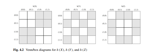
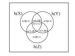
One fair die is thrown first and the result is recorded odd as 1 (the number of the face up mod 2) or even as 0 . Then the same is done with a second fair die so the outcome space if $U={(0,0),(0,1),(1,0),(1,1)}={0,1} \times{0,1}$ (first die on the left and second die on the right). Let $X$ be the random variable for the outcome ( 0 or 1 ) of the first throw, $Y$ for the second throw, and $Z$ for the sum $X+Y$ mod 2. Since $Z$ is a function of $X$ and $Y$, the outcome space is $U \times U=(X \times Y)^{2}$. So many Venn diagrams are illustrated rather symbolically, e.g., with circles for $h(X)$, $h(Y)$, and $h(Z)$, that it will be useful to give the actual Venn/box diagrams for this example.
The two-draw outcome space $U \times U$ can be represented as a $4 \times 4$ square with each square representing a point $\left((x, y),\left(x^{\prime}, y^{\prime}\right)\right)$ for the two trials with the dice. The points included in $h(X)$ (indicated with shading) are the pairs $\left((x, y),\left(x^{\prime}, y^{\prime}\right)\right)$ where $x \neq x^{\prime}$ and symmetrically for $h(Y)$. Since $Z=X+Y \bmod 2$, the shaded squares for $h(Z)$ are the squares $\left((x, y),\left(x^{\prime}, y^{\prime}\right)\right)$ where $x+y \neq x^{\prime}+y^{\prime} \bmod 2$ as shown in Fig. 4.2.
Since each point in $U \times U$ has the product probability $\frac{1}{4} \times \frac{1}{4}=\frac{1}{16}$ and the logical entropies are just the sum of the probabilities of the shaded squares, we see that $h(X)=h(Y)=h(Z)=\frac{8}{16}=\frac{1}{2}$. The joint logical entropies are the sum of the probabilities for the squares that are shaded in one or the other (or both) shown in Fig. $4.3$.
数学代写|信息论代写information theory代考|Entropies for Countable Probability Distributions
The logical entropies for any discrete probability distributions, finite or countably infinite, can be illustrated with an logical entropy box diagram. A square with unit length sides can have the probabilities $p_{1}, p_{2} \ldots .$ marked off along the width and height so that squares $p_{i}^{2}$ and products $p_{i} p_{j}$ and $p_{j} p_{i}$ all correspond to the area of rectangles in the square. The sum of the square areas along the diagonal is $\sum_{i} p_{i}^{2}$ so the logical entropy $h(p)=1-\sum_{i} p_{i}^{2}$ is the sum of the two equal areas of rectangles on either side of the diagonal. Figure $4.7$ gives the logical entropy box diagram for the countable distribution, $p_{1}=\frac{1}{2}, p_{2}=\left(\frac{1}{2}\right)^{2}, \ldots, p_{n}=\left(\frac{1}{2}\right)^{n}, \ldots$ which sums to 1 .
Since $\sum_{i} p_{i}=1$, the logical entropy $h(p)=1-\sum_{i} p_{i}^{2}$ for countable distributions is always well-defined, strictly less than one, and interpretable as the two-draw probability of getting different indices $i \neq j$. However, the Shannon entropy for countable distributions $H(p)=\sum_{i} p_{i} \log {2}\left(\frac{1}{p{i}}\right)$ may blow up (not have a finite sum); examples are given in [23, Example 2.46, p. 30] and [6, p. 48].
For the example at hand, the sum of the probabilities squared is $\frac{1}{4}+\frac{1}{16}+\frac{1}{64}+\ldots=$ $\left(\frac{1}{4}\right)^{1}+\left(\frac{1}{4}\right)^{2}+\left(\frac{1}{4}\right)^{3}+\ldots=\frac{1 / 4}{1-1 / 4}=\frac{1}{3}$ (the area of the diagonal squares in the box diagram of Fig. 4.7) so the logical entropy is $h(p)=1-\frac{1}{3}=\frac{2}{3}$. In the box diagram with a uniform distribution over the unit area, the logical entropy is the probability that a random point in the square lies off the boxed diagonal.
信息论代考
数学代写|信息论代写information theory代考|Entropies for Multivariate Joint Distributions
让\left{p\left(x_{1}, \ldots, x_{n}\right)\right}\left{p\left(x_{1}, \ldots, x_{n}\right)\right}是一个概率分布X1×…×Xn对于有限X一世的。让小号成为的一个子集(X1×…×Xn)2由某些有序的有序对组成n-元组((X1,…,Xn),(X1′,…,Xn′))所以产品概率测度小号是:
\mu(S)=\sum\left{p\left(x_{1}, \ldots, x_{n}\right) p\left(x_{1}^{\prime}, \ldots, x_{n }^{\prime}\right):\left(\left(x_{1}, \ldots, x_{n}\right),\left(x_{1}^{\prime}, \ldots, x_{ n}^{\prime}\right)\right) \in S\right}\mu(S)=\sum\left{p\left(x_{1}, \ldots, x_{n}\right) p\left(x_{1}^{\prime}, \ldots, x_{n }^{\prime}\right):\left(\left(x_{1}, \ldots, x_{n}\right),\left(x_{1}^{\prime}, \ldots, x_{ n}^{\prime}\right)\right) \in S\right}
然后是这个的所有逻辑熵n- 变量案例作为某些信息集的产品度量给出小号. 让我,Ĵ⊆ñ是所有变量集合的子集N=\left{X_{1}, \ldots, X_{n}\right}N=\left{X_{1}, \ldots, X_{n}\right}然后让X=(X1,…,Xn)和X′=(X1′,…,Xn′).
由于两个订购n-如果元组在某个坐标上不同,则它们是不同的,所有变量的联合逻辑熵为:H(X1,…,Xn)=μ(小号在ñ)在哪里:
\begin{聚集} S_{\vee N}=\left{\left(x, x^{\prime}\right): \vee_{i=1}^{n}\left(x_{i} \neq x_{i}^{\prime}\right)\right}=\cup\left{S_{X_{i}}: X_{i} \in N\right} \text { where } \ S_{X_{i }}=S_{x_{i} \neq x_{i}^{\prime}}=\left{\left(x, x^{\prime}\right): x_{i} \neq x_{i} ^{\prime}\right} \end{聚集}\begin{聚集} S_{\vee N}=\left{\left(x, x^{\prime}\right): \vee_{i=1}^{n}\left(x_{i} \neq x_{i}^{\prime}\right)\right}=\cup\left{S_{X_{i}}: X_{i} \in N\right} \text { where } \ S_{X_{i }}=S_{x_{i} \neq x_{i}^{\prime}}=\left{\left(x, x^{\prime}\right): x_{i} \neq x_{i} ^{\prime}\right} \end{聚集}
(在哪里∨表示语句的析取)。对于非空我⊆ñ, 中变量的联合逻辑熵我可以表示为H(我)=μ(小号∨我)在哪里:
S_{\vee I}=\left{\left(x, x^{\prime}\right): \vee\left(x_{i} \neq x_{i}^{\prime}\right) \text { for } X_{i} \in I\right}=\cup\left{S_{X_{i}}: X_{i} \in I\right}S_{\vee I}=\left{\left(x, x^{\prime}\right): \vee\left(x_{i} \neq x_{i}^{\prime}\right) \text { for } X_{i} \in I\right}=\cup\left{S_{X_{i}}: X_{i} \in I\right}
以便H(X1,…,Xn)=H(ñ).
和以前一样,信息代数我(X1×…×Xn)是的布尔子代数℘((X1×…×Xn)2)由基本信息集生成小号X一世对于变量及其补码小号¬XF.
对于条件逻辑熵,让我,Ĵ⊆ñ是两个非空不相交子集ñ. 条件熵的概念H(我∣Ĵ)是表示变量中的信息我由定义条件给出:∨(X一世≠X一世′)为了X一世∈我, 去掉变量中的信息后Ĵ这由条件定义:∨(Xj≠Xj′)为了Xj∈Ĵ. “酒吧之后∣”的意思是“否定”,所以我们否定那个条件∨(Xj≠Xj′)为了Xj∈Ĵ并将其添加到条件中我获得条件逻辑熵为H(我∣Ĵ)=H(∨我∣∨Ĵ)=μ(小号∨我∣∨Ĵ)(在哪里∧表示语句的合取):
\begin{对齐} S_{\vee I \mid \vee J}=&\left{\left(x, x^{\prime}\right): \vee\left(x_{i} \neq x_{i }^{\prime}\right) \text { for } X_{i} \in I \text { 和 } \wedge\left(x_{j}=x_{j}^{\prime}\right) \text { for } X_{j} \in J\right} \ &=\cup\left{S_{X_{i}}: X_{i} \in I\right}-\cup\left{S_{X_{j }}: X_{j} \in J\right}=S_{\vee I}-S_{\vee J} \end{aligned}\begin{对齐} S_{\vee I \mid \vee J}=&\left{\left(x, x^{\prime}\right): \vee\left(x_{i} \neq x_{i }^{\prime}\right) \text { for } X_{i} \in I \text { 和 } \wedge\left(x_{j}=x_{j}^{\prime}\right) \text { for } X_{j} \in J\right} \ &=\cup\left{S_{X_{i}}: X_{i} \in I\right}-\cup\left{S_{X_{j }}: X_{j} \in J\right}=S_{\vee I}-S_{\vee J} \end{aligned}
数学代写|信息论代写information theory代考|An Example of Negative Mutual Information
Norman Abramson 给出了一个示例 [1, pp. 130-131],其中三个变量的香农互信息为负。3William Feller 给出了一个类似的具体示例,我们将使用该示例 [11, 练习 26, p. 143]。任何表明成对独立并不意味着三个或更多随机变量的相互独立的概率论教科书示例也可以。
首先抛出一个公平骰子,结果记录为奇数为 1(正面朝上的数字 2)或偶数为 0 。然后用第二个公平骰子做同样的事情,所以结果空间如果在=(0,0),(0,1),(1,0),(1,1)=0,1×0,1(左边第一个骰子,右边第二个骰子)。让X是第一次投掷结果( 0 或 1 )的随机变量,是第二次投掷,和从总和X+是mod 2. 因为从是一个函数X和是,结果空间为在×在=(X×是)2. 如此多的维恩图是用象征性的方式来说明的,例如,用圆圈表示H(X), H(是), 和H(从),给出这个例子的实际维恩/箱形图会很有用。
两次抽签结果空间在×在可以表示为4×4正方形,每个正方形代表一个点((X,是),(X′,是′))对于骰子的两次试验。包含的点数H(X)(用阴影表示)是对((X,是),(X′,是′))在哪里X≠X′并且对称地为H(是). 自从从=X+是反对2,阴影方块为H(从)是正方形((X,是),(X′,是′))在哪里X+是≠X′+是′反对2如图 4.2 所示。
由于每个点在×在有乘积概率14×14=116并且逻辑熵只是阴影方块的概率之和,我们看到H(X)=H(是)=H(从)=816=12. 联合逻辑熵是在图 1 中显示的一个或另一个(或两个)阴影中的正方形的概率之和。4.3.
数学代写|信息论代写information theory代考|Entropies for Countable Probability Distributions
任何离散概率分布(有限或可数无限)的逻辑熵都可以用逻辑熵箱图来说明。具有单位长度边的正方形可以有概率p1,p2….沿宽度和高度标出,使正方形p一世2和产品p一世pj和pjp一世都对应于正方形中长方形的面积。沿对角线的正方形面积之和为∑一世p一世2所以逻辑熵H(p)=1−∑一世p一世2是对角线两侧的两个相等的矩形面积之和。数字4.7给出可数分布的逻辑熵箱图,p1=12,p2=(12)2,…,pn=(12)n,…总和为 1 。
自从∑一世p一世=1, 逻辑熵H(p)=1−∑一世p一世2对于可数分布总是定义明确的,严格小于一,并且可以解释为获得不同指数的两次抽签概率一世≠j. 然而,可数分布的香农熵H(p)=∑一世p一世日志2(1p一世)可能会爆炸(没有有限的总和);示例在 [23, Example 2.46, p. 30] 和 [6, p. 48]。
对于手头的示例,概率平方和为14+116+164+…= (14)1+(14)2+(14)3+…=1/41−1/4=13(图 4.7 方框图中对角线方块的面积)所以逻辑熵是H(p)=1−13=23. 在单位面积上均匀分布的箱形图中,逻辑熵是正方形中随机点位于盒装对角线之外的概率。

统计代写请认准statistics-lab™. statistics-lab™为您的留学生涯保驾护航。
金融工程代写
金融工程是使用数学技术来解决金融问题。金融工程使用计算机科学、统计学、经济学和应用数学领域的工具和知识来解决当前的金融问题,以及设计新的和创新的金融产品。
非参数统计代写
非参数统计指的是一种统计方法,其中不假设数据来自于由少数参数决定的规定模型;这种模型的例子包括正态分布模型和线性回归模型。
广义线性模型代考
广义线性模型(GLM)归属统计学领域,是一种应用灵活的线性回归模型。该模型允许因变量的偏差分布有除了正态分布之外的其它分布。
术语 广义线性模型(GLM)通常是指给定连续和/或分类预测因素的连续响应变量的常规线性回归模型。它包括多元线性回归,以及方差分析和方差分析(仅含固定效应)。
有限元方法代写
有限元方法(FEM)是一种流行的方法,用于数值解决工程和数学建模中出现的微分方程。典型的问题领域包括结构分析、传热、流体流动、质量运输和电磁势等传统领域。
有限元是一种通用的数值方法,用于解决两个或三个空间变量的偏微分方程(即一些边界值问题)。为了解决一个问题,有限元将一个大系统细分为更小、更简单的部分,称为有限元。这是通过在空间维度上的特定空间离散化来实现的,它是通过构建对象的网格来实现的:用于求解的数值域,它有有限数量的点。边界值问题的有限元方法表述最终导致一个代数方程组。该方法在域上对未知函数进行逼近。[1] 然后将模拟这些有限元的简单方程组合成一个更大的方程系统,以模拟整个问题。然后,有限元通过变化微积分使相关的误差函数最小化来逼近一个解决方案。
tatistics-lab作为专业的留学生服务机构,多年来已为美国、英国、加拿大、澳洲等留学热门地的学生提供专业的学术服务,包括但不限于Essay代写,Assignment代写,Dissertation代写,Report代写,小组作业代写,Proposal代写,Paper代写,Presentation代写,计算机作业代写,论文修改和润色,网课代做,exam代考等等。写作范围涵盖高中,本科,研究生等海外留学全阶段,辐射金融,经济学,会计学,审计学,管理学等全球99%专业科目。写作团队既有专业英语母语作者,也有海外名校硕博留学生,每位写作老师都拥有过硬的语言能力,专业的学科背景和学术写作经验。我们承诺100%原创,100%专业,100%准时,100%满意。
随机分析代写
随机微积分是数学的一个分支,对随机过程进行操作。它允许为随机过程的积分定义一个关于随机过程的一致的积分理论。这个领域是由日本数学家伊藤清在第二次世界大战期间创建并开始的。
时间序列分析代写
随机过程,是依赖于参数的一组随机变量的全体,参数通常是时间。 随机变量是随机现象的数量表现,其时间序列是一组按照时间发生先后顺序进行排列的数据点序列。通常一组时间序列的时间间隔为一恒定值(如1秒,5分钟,12小时,7天,1年),因此时间序列可以作为离散时间数据进行分析处理。研究时间序列数据的意义在于现实中,往往需要研究某个事物其随时间发展变化的规律。这就需要通过研究该事物过去发展的历史记录,以得到其自身发展的规律。
回归分析代写
多元回归分析渐进(Multiple Regression Analysis Asymptotics)属于计量经济学领域,主要是一种数学上的统计分析方法,可以分析复杂情况下各影响因素的数学关系,在自然科学、社会和经济学等多个领域内应用广泛。
MATLAB代写
MATLAB 是一种用于技术计算的高性能语言。它将计算、可视化和编程集成在一个易于使用的环境中,其中问题和解决方案以熟悉的数学符号表示。典型用途包括:数学和计算算法开发建模、仿真和原型制作数据分析、探索和可视化科学和工程图形应用程序开发,包括图形用户界面构建MATLAB 是一个交互式系统,其基本数据元素是一个不需要维度的数组。这使您可以解决许多技术计算问题,尤其是那些具有矩阵和向量公式的问题,而只需用 C 或 Fortran 等标量非交互式语言编写程序所需的时间的一小部分。MATLAB 名称代表矩阵实验室。MATLAB 最初的编写目的是提供对由 LINPACK 和 EISPACK 项目开发的矩阵软件的轻松访问,这两个项目共同代表了矩阵计算软件的最新技术。MATLAB 经过多年的发展,得到了许多用户的投入。在大学环境中,它是数学、工程和科学入门和高级课程的标准教学工具。在工业领域,MATLAB 是高效研究、开发和分析的首选工具。MATLAB 具有一系列称为工具箱的特定于应用程序的解决方案。对于大多数 MATLAB 用户来说非常重要,工具箱允许您学习和应用专业技术。工具箱是 MATLAB 函数(M 文件)的综合集合,可扩展 MATLAB 环境以解决特定类别的问题。可用工具箱的领域包括信号处理、控制系统、神经网络、模糊逻辑、小波、仿真等。