如果你也在 怎样代写拓扑学Topology这个学科遇到相关的难题,请随时右上角联系我们的24/7代写客服。
拓扑学是数学的一个分支,有时被称为 “橡胶板几何”,在这个分支中,如果两个物体可以通过弯曲、扭曲、拉伸和收缩等空间运动连续变形为彼此,同时不允许撕开或粘在一起的部分,则被认为是等效的。
statistics-lab™ 为您的留学生涯保驾护航 在代写拓扑学Topology方面已经树立了自己的口碑, 保证靠谱, 高质且原创的统计Statistics代写服务。我们的专家在代写拓扑学Topology代写方面经验极为丰富,各种代写拓扑学Topology相关的作业也就用不着说。
我们提供的拓扑学Topology及其相关学科的代写,服务范围广, 其中包括但不限于:
- Statistical Inference 统计推断
- Statistical Computing 统计计算
- Advanced Probability Theory 高等概率论
- Advanced Mathematical Statistics 高等数理统计学
- (Generalized) Linear Models 广义线性模型
- Statistical Machine Learning 统计机器学习
- Longitudinal Data Analysis 纵向数据分析
- Foundations of Data Science 数据科学基础
数学代写|拓扑学代写Topology代考|Adjoint Analysis for Electric Field-Based Topology
The Lagrangian multiplier-based adjoint sensitivity analysis of variational problem in Eq. $3.23$ is implemented as follows. The functional space and trace operators of Eq. 3.14 are similarly defined as that in Sect. 3.1.2, except that
$$
\mathscr{V}{\mathbf{E}} \doteq\left{\mathbf{u} \in \mathscr{H}(\operatorname{curl} ; \Omega) \mid \nabla \cdot \mathbf{u}=0, \text { in } \Omega ; \mathbf{n} \times \mathbf{u}=\mathbf{0} \text {, on } \Gamma{P E C}\right}
$$
According to the Kurash-Kuhn-Tucker condition of the PDE constrained optimization problem [22], the adjoint equations can be obtained as
Find $\mathbf{E}{s a} \in \mathscr{V}{\mathbf{E}}$ such that
$$
\begin{aligned}
&\int_{\Omega} \frac{\partial A}{\partial \mathbf{E}{s}} \cdot \phi+\frac{\partial A}{\partial \nabla \times \mathbf{E}{s}} \cdot(\nabla \times \phi)+\mu_{r}^{-1}\left(\nabla \times \overline{\mathbf{E}}{s a}\right) \cdot(\nabla \times \phi)-k{0}^{2} \varepsilon_{r} \overline{\mathbf{E}}{s a} \cdot \phi \mathrm{d} \Omega \ &+\int{\Gamma_{a}} j k_{0} \sqrt{\varepsilon_{r} \mu_{r}^{-1}}\left(\mathbf{n} \times \overline{\mathbf{E}}{s a} \times \mathbf{n}\right) \cdot(\mathbf{n} \times \phi \times \mathbf{n})+\frac{\partial B}{\partial \mathbf{E}{s}} \cdot \phi \mathrm{d} \Gamma \
&+\int_{\Gamma_{P M c}} \frac{\partial B}{\partial \mathbf{E}{s}} \cdot \phi \mathrm{d} \Gamma=0, \forall \phi \in \mathscr{V}{\mathbf{E}} \
&\text { Find } \gamma_{f a} \in \mathscr{H}(\Omega) \text { such that } \
&\int_{\Omega} r^{2} \nabla_{\gamma_{f a}} \cdot \nabla \phi+\gamma_{f a} \phi+A_{\gamma_{e}} \phi-S_{\gamma_{c}} \phi \mathrm{d} \Omega=0, \forall \phi \in \mathscr{H}(\Omega)
\end{aligned}
$$
where $A_{\gamma_{c}}(\Omega)$ is defined as
$$
A_{\gamma_{e}}=\sum_{n=1}^{N} A_{\gamma_{n e}}\left(\Omega_{n}\right)
$$
with
$$
A_{\gamma_{n e s}}\left(\Omega_{n}\right)=\left{\begin{array}{l}
\frac{1}{V_{\Omega_{n}}} \int_{\Omega_{n}} \frac{\partial A}{\partial \gamma_{p}} \frac{\partial \gamma_{p}}{\partial \gamma_{e}} \mathrm{~d} \Omega, \forall \mathbf{x} \in \Omega_{n} \
0, \forall \mathbf{x} \in \Omega \backslash \Omega_{n}
\end{array}\right.
$$
and $S_{\gamma_{c}}(\Omega)$ is defined to be
$$
S_{\gamma_{e}}=\sum_{n=1}^{N} S_{\gamma_{a, e}}\left(\Omega_{n}\right)
$$
with
$$
S_{\gamma_{n, c}}\left(\Omega_{n}\right)=\left{\begin{array}{l}
\frac{1}{V_{\Omega_{n}}} \int_{\Omega_{n}} k_{0}^{2} \frac{\partial \varepsilon_{r}}{\partial \gamma_{p}} \frac{\partial \gamma_{p}}{\partial \gamma_{e}}\left(\mathbf{E}{s}+\mathbf{E}{i}\right) \cdot \overline{\mathbf{E}}{s a} \mathrm{~d} \Omega, \forall \mathbf{x} \in \Omega{n} \
0, \forall \mathbf{x} \in \Omega \backslash \Omega_{n}
\end{array}\right.
$$
The adjoint derivative of the cost functional can be derived as
$$
\delta J=\int_{\Omega} \operatorname{Re}\left(\frac{\partial A}{\partial \gamma}-\bar{\gamma}_{f a}\right) \delta \gamma \mathrm{d} \Omega
$$
数学代写|拓扑学代写Topology代考|Numerical implementation
In the wave equations and corresponding adjoint equations, a divergence-free condition needs to be satisfied for both the state variable and the adjoint variable. Therefore,
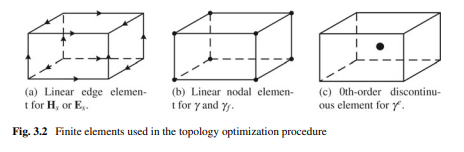
the edge element-based finite element method is utilized to solve the wave equations and adjoint equations, where brick elements are used to discretize the computational domain and simultaneously ensure the divergence-free condition [28]. For the Helmholtz filter, the filter Eq. $3.4$ and its adjoint equation are solved using the standard Galerkin finite element method.
The topology optimization method for three-dimensional optical waves is implemented by a gradient-based iterative procedure, where the gradient information is derived by sensitivity analysis as demonstrated in Sects. 3.1.2 and 3.1.4 respectively corresponding to the variational problems in Eqs.3.7 and 3.23. The flowcharts for iteratively solving the variational problems (Eqs. $3.7$ and $3.23$ ) respectively corresponding to the magnetic field formulation and electric field formulation are respectively shown in Fig. 3.1a and b. The iterative procedure includes the following steps: (a) solve the wave equations with the current design variable; (b) solve the adjoint equations based on the solution of the wave equations; (c) compute the adjoint derivative of the design objective; and (d) update the design variable using the method of moving asymptotes [47].
During the solving procedure, the filter radius $r$ of the Helmholtz filter in Eq.3.4 is set to be the size of the finite elements used to discretize the computational domain; the threshold parameter $\xi$ in Eqs. $3.5$ and $3.21$ is set to be $0.5$; the initial value of the projection parameter $\beta$ is set to be 1 and it is doubled after every fixed number of iterations until the preset maximal value $2^{10}$ is reached (eleven cycles). The above steps are implemented iteratively until the stopping criterion is satisfied, specified to be the change of the objective values in five consecutive iterations satisfying
$$
\frac{1}{5} \sum_{i=1}^{4}\left|J_{k-i}-J_{k-i-1}\right| /\left|J_{k}\right| \leq \varepsilon, \beta \geq 2^{10}
$$
in the $k$ th iteration, where $J_{k}$ is the objective value computed in the $k$ th iteration; $\varepsilon$ is the tolerance chosen to be $1 \times 10^{-3}$. Because the iteration number is set to be 40 before doubling the projection parameter, the maximal iterative number is set to be $440 .$
In the optimization procedure for magnetic field described optical waves, the magnetic field is interpolated using linear edge elements (Fig. 3.2a); the design variable and filtered design variable is interpolated using linear nodal element (Fig. 3.2b). In the optimization procedure for electric field described optical waves, the electric field is interpolated using linear edge elements (Fig. 3.2a); the design variable and filtered design variable is interpolated using linear nodal elements (Fig. 3.2b); the filtered design variable is converted to piecewise form by interpolating the piecewise design variable using zeroth-order discontinuous elements (Fig. $3.2 \mathrm{c}$ ), where $\Omega_{n}$ in Eq. $3.20$ is set to be the space taken up by the brick elements.
数学代写|拓扑学代写Topology代考|Cloak for Perfect Conductor
The cloaks for perfect conductor are inversely designed using the developed method. This is a typical min-type optimization problem. Topology optimization-based inverse design of two-dimensional optical cloaks have been investigated for transverse magnetic and transverse electric incident waves, where two-dimensional is the reduced case with an infinite extension assumed in the third dimension $[3,4$, 16]. Three-dimensional design is more flexible and practical for the consideration of realistic situations.
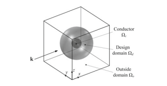
In the following, optical cloaks are designed for a spherical perfect conductor. To cloak the sphere, the scattering field should be minimized to achieve phase matching of the total field around the conductor. The inverse domain of the cloak is set to be a cube with side length equal to 7 times the incident wavelength, as shown in Fig. 3.3, where the cloak domain is set to be a spherical shell with external and internal radii equal to $2.5$ and $0.75$ times the incident wavelength, and the cloaked conductor is enclosed in a central spherical domain with a radius equal to $0.75$ times the incident wavelength. The computational domain is discretized by $63 \times 63 \times 63$ brick elements.
For a magnetic field described optical cloak, the objective in Eq. $3.8$ is set to minimize the normalized square norm of the scattered magnetic field
$$
J=\frac{1}{J_{0}} \int_{\Omega_{a}} \mathbf{H}{s} \cdot \overline{\mathbf{H}}{s} \mathrm{~d} \Omega
$$
where $\Omega_{o}$ is the domain outside the spherical shell-shaped design domain; $J_{0}$ is the square norm of the uncloaked scattered magnetic field in the outside domain of the cloak. The obtained cloak topology, found by solving the corresponding topology optimization problem, is shown in Fig. 3.4a, with incident wave, uncloaked field, and cloaked field shown in Fig. $3.4 \mathrm{c}$, d, and e, where the incident wave is set to be the uniform plane wave $\mathbf{H}{i}=\left(0,0, e^{-j k{0} x}\right)$ with $k_{0}=20 \pi \mathrm{rad} / \mathrm{m}$. For an electric field described optical cloak, the objective in Eq. $3.24$ is set to minimize the normalized square norm of the scattered electric field
$$
J=\frac{1}{J_{0}} \int_{\Omega_{o}} \mathbf{E}{s} \cdot \overline{\mathbf{E}}{s} \mathrm{~d} \Omega
$$
拓扑学代考
数学代写|拓扑学代写Topology代考|Adjoint Analysis for Electric Field-Based Topology
方程中变分问题的基于拉格朗日乘数的伴随敏感性分析。3.23实现如下。方程的函数空间和迹算子。3.14 的定义与第 3.14 节中的定义类似。3.1.2,除了
\mathscr{V}{\mathbf{E}} \doteq\left{\mathbf{u} \in \mathscr{H}(\operatorname{curl} ; \Omega) \mid \nabla \cdot \mathbf{u} =0, \text { } \Omega ; \mathbf{n} \times \mathbf{u}=\mathbf{0} \text {, on } \Gamma{PEC}\right}\mathscr{V}{\mathbf{E}} \doteq\left{\mathbf{u} \in \mathscr{H}(\operatorname{curl} ; \Omega) \mid \nabla \cdot \mathbf{u} =0, \text { } \Omega ; \mathbf{n} \times \mathbf{u}=\mathbf{0} \text {, on } \Gamma{PEC}\right}
根据 PDE 约束优化问题 [22] 的 Kurash-Kuhn-Tucker 条件,可以得到伴随方程为
寻找和s一个∈在和这样
∫Ω∂一个∂和s⋅φ+∂一个∂∇×和s⋅(∇×φ)+μr−1(∇×和¯s一个)⋅(∇×φ)−ķ02er和¯s一个⋅φdΩ +∫Γ一个jķ0erμr−1(n×和¯s一个×n)⋅(n×φ×n)+∂乙∂和s⋅φdΓ +∫Γ磷米C∂乙∂和s⋅φdΓ=0,∀φ∈在和 寻找 CF一个∈H(Ω) 这样 ∫Ωr2∇CF一个⋅∇φ+CF一个φ+一个C和φ−小号CCφdΩ=0,∀φ∈H(Ω)
在哪里一个CC(Ω)定义为
一个C和=∑n=1ñ一个Cn和(Ωn)
$$ A_{\ gamma_
{nes}}\left(\Omega_{n}\right)=\left{
1在Ωn∫Ωn∂一个∂Cp∂Cp∂C和 dΩ,∀X∈Ωn 0,∀X∈Ω∖Ωn\正确的。
一个nd$小号CC(Ω)$一世sd和F一世n和d吨○b和
S_{\gamma_{e}}=\sum_{n=1}^{N} S_{\gamma_{a, e}}\left(\Omega_{n}\right)
在一世吨H
S_{\gamma_{n, c}}\left(\Omega_{n}\right)=\left{
1在Ωn∫Ωnķ02∂er∂Cp∂Cp∂C和(和s+和一世)⋅和¯s一个 dΩ,∀X∈Ωn 0,∀X∈Ω∖Ωn\正确的。
吨H和一个dj○一世n吨d和r一世在一个吨一世在和○F吨H和C○s吨F在nC吨一世○n一个lC一个nb和d和r一世在和d一个s
\delta J=\int_{\Omega} \operatorname{Re}\left(\frac{\partial A}{\partial \gamma}-\bar{\gamma}_{fa}\right) \delta \gamma\数学{d}\欧米茄
$$
数学代写|拓扑学代写Topology代考|Numerical implementation
在波动方程和相应的伴随方程中,状态变量和伴随变量都需要满足无散条件。所以,
基于边缘元的有限元方法用于求解波动方程和伴随方程,其中砖元用于离散计算域并同时确保无散度条件[28]。对于亥姆霍兹滤波器,滤波器方程。3.4及其伴随方程使用标准 Galerkin 有限元方法求解。
三维光波的拓扑优化方法是通过基于梯度的迭代过程实现的,其中梯度信息是通过灵敏度分析得出的,如 Sects 所示。3.1.2 和 3.1.4 分别对应方程 3.7 和 3.23 中的变分问题。迭代求解变分问题的流程图(方程式。3.7和3.23) 分别对应的磁场公式和电场公式分别如图 3.1a 和 b 所示。迭代过程包括以下步骤: (a) 用当前设计变量求解波动方程;(b) 在求解波动方程的基础上求解伴随方程;(c) 计算设计目标的伴随导数;(d) 使用移动渐近线的方法更新设计变量[47]。
在求解过程中,滤波器半径rEq.3.4 中的亥姆霍兹滤波器的大小被设置为用于离散计算域的有限元的大小;阈值参数X在方程式中。3.5和3.21设置为0.5; 投影参数的初始值b设置为1,每固定迭代次数加倍,直到预设最大值210达到(十一个周期)。上述步骤迭代执行,直到满足停止准则,指定为连续五次迭代中目标值的变化满足
15∑一世=14|Ĵķ−一世−Ĵķ−一世−1|/|Ĵķ|≤e,b≥210
在里面ķ第一次迭代,其中Ĵķ是计算的目标值ķ第一次迭代;e是选择的公差1×10⁻³. 因为在投影参数加倍之前迭代次数设置为40,所以最大迭代次数设置为440.
在磁场描述的光波的优化过程中,使用线性边缘元素对磁场进行插值(图 3.2a);设计变量和过滤设计变量使用线性节点元素进行插值(图 3.2b)。在电场描述光波的优化过程中,使用线性边缘元素对电场进行插值(图 3.2a);设计变量和过滤设计变量使用线性节点元素进行插值(图 3.2b);通过使用零阶不连续元素对分段设计变量进行插值,将过滤后的设计变量转换为分段形式(图 3)。3.2C), 在哪里Ωn在等式。3.20设置为砖元素占用的空间。
数学代写|拓扑学代写Topology代考|Cloak for Perfect Conductor
完美导体的斗篷是使用开发的方法逆向设计的。这是一个典型的 min-type 优化问题。已经研究了基于拓扑优化的二维光学斗篷的逆向设计,用于横向磁和横向电入射波,其中二维是在第三维中假设无限扩展的简化情况[3,4, 16]。立体设计更加灵活实用,考虑到现实情况。
在下文中,光学斗篷是为球形完美导体设计的。为了掩盖球体,散射场应该最小化,以实现导体周围总场的相位匹配。斗篷的逆域设置为边长等于入射波长的 7 倍的立方体,如图 3.3 所示,其中斗篷域设置为外半径和内半径等于的球壳2.5和0.75乘以入射波长,隐形导体被包围在一个半径等于0.75乘以入射波长。计算域离散化为63×63×63砖元素。
对于磁场描述的光学斗篷,方程式中的物镜。3.8设置为最小化散射磁场的归一化平方范数
Ĵ=1Ĵ0∫Ω一个Hs⋅H¯s dΩ
在哪里Ω○是球壳形设计域外的域;Ĵ0是斗篷外域中未隐身散射磁场的平方范数。通过求解相应的拓扑优化问题得到的隐身拓扑如图3.4a所示,入射波、非隐身场和隐身场如图3.4a所示。3.4C, d, 和 e,其中入射波设置为均匀平面波H一世=(0,0,和−jķ0X)和ķ0=20圆周率r一个d/米. 对于电场描述的光学斗篷,方程式中的物镜。3.24设置为最小化散射电场的归一化平方范数
Ĵ=1Ĵ0∫Ω○和s⋅和¯s dΩ

统计代写请认准statistics-lab™. statistics-lab™为您的留学生涯保驾护航。
金融工程代写
金融工程是使用数学技术来解决金融问题。金融工程使用计算机科学、统计学、经济学和应用数学领域的工具和知识来解决当前的金融问题,以及设计新的和创新的金融产品。
非参数统计代写
非参数统计指的是一种统计方法,其中不假设数据来自于由少数参数决定的规定模型;这种模型的例子包括正态分布模型和线性回归模型。
广义线性模型代考
广义线性模型(GLM)归属统计学领域,是一种应用灵活的线性回归模型。该模型允许因变量的偏差分布有除了正态分布之外的其它分布。
术语 广义线性模型(GLM)通常是指给定连续和/或分类预测因素的连续响应变量的常规线性回归模型。它包括多元线性回归,以及方差分析和方差分析(仅含固定效应)。
有限元方法代写
有限元方法(FEM)是一种流行的方法,用于数值解决工程和数学建模中出现的微分方程。典型的问题领域包括结构分析、传热、流体流动、质量运输和电磁势等传统领域。
有限元是一种通用的数值方法,用于解决两个或三个空间变量的偏微分方程(即一些边界值问题)。为了解决一个问题,有限元将一个大系统细分为更小、更简单的部分,称为有限元。这是通过在空间维度上的特定空间离散化来实现的,它是通过构建对象的网格来实现的:用于求解的数值域,它有有限数量的点。边界值问题的有限元方法表述最终导致一个代数方程组。该方法在域上对未知函数进行逼近。[1] 然后将模拟这些有限元的简单方程组合成一个更大的方程系统,以模拟整个问题。然后,有限元通过变化微积分使相关的误差函数最小化来逼近一个解决方案。
tatistics-lab作为专业的留学生服务机构,多年来已为美国、英国、加拿大、澳洲等留学热门地的学生提供专业的学术服务,包括但不限于Essay代写,Assignment代写,Dissertation代写,Report代写,小组作业代写,Proposal代写,Paper代写,Presentation代写,计算机作业代写,论文修改和润色,网课代做,exam代考等等。写作范围涵盖高中,本科,研究生等海外留学全阶段,辐射金融,经济学,会计学,审计学,管理学等全球99%专业科目。写作团队既有专业英语母语作者,也有海外名校硕博留学生,每位写作老师都拥有过硬的语言能力,专业的学科背景和学术写作经验。我们承诺100%原创,100%专业,100%准时,100%满意。
随机分析代写
随机微积分是数学的一个分支,对随机过程进行操作。它允许为随机过程的积分定义一个关于随机过程的一致的积分理论。这个领域是由日本数学家伊藤清在第二次世界大战期间创建并开始的。
时间序列分析代写
随机过程,是依赖于参数的一组随机变量的全体,参数通常是时间。 随机变量是随机现象的数量表现,其时间序列是一组按照时间发生先后顺序进行排列的数据点序列。通常一组时间序列的时间间隔为一恒定值(如1秒,5分钟,12小时,7天,1年),因此时间序列可以作为离散时间数据进行分析处理。研究时间序列数据的意义在于现实中,往往需要研究某个事物其随时间发展变化的规律。这就需要通过研究该事物过去发展的历史记录,以得到其自身发展的规律。
回归分析代写
多元回归分析渐进(Multiple Regression Analysis Asymptotics)属于计量经济学领域,主要是一种数学上的统计分析方法,可以分析复杂情况下各影响因素的数学关系,在自然科学、社会和经济学等多个领域内应用广泛。
MATLAB代写
MATLAB 是一种用于技术计算的高性能语言。它将计算、可视化和编程集成在一个易于使用的环境中,其中问题和解决方案以熟悉的数学符号表示。典型用途包括:数学和计算算法开发建模、仿真和原型制作数据分析、探索和可视化科学和工程图形应用程序开发,包括图形用户界面构建MATLAB 是一个交互式系统,其基本数据元素是一个不需要维度的数组。这使您可以解决许多技术计算问题,尤其是那些具有矩阵和向量公式的问题,而只需用 C 或 Fortran 等标量非交互式语言编写程序所需的时间的一小部分。MATLAB 名称代表矩阵实验室。MATLAB 最初的编写目的是提供对由 LINPACK 和 EISPACK 项目开发的矩阵软件的轻松访问,这两个项目共同代表了矩阵计算软件的最新技术。MATLAB 经过多年的发展,得到了许多用户的投入。在大学环境中,它是数学、工程和科学入门和高级课程的标准教学工具。在工业领域,MATLAB 是高效研究、开发和分析的首选工具。MATLAB 具有一系列称为工具箱的特定于应用程序的解决方案。对于大多数 MATLAB 用户来说非常重要,工具箱允许您学习和应用专业技术。工具箱是 MATLAB 函数(M 文件)的综合集合,可扩展 MATLAB 环境以解决特定类别的问题。可用工具箱的领域包括信号处理、控制系统、神经网络、模糊逻辑、小波、仿真等。