如果你也在 怎样代写有限元方法Finite Element Method这个学科遇到相关的难题,请随时右上角联系我们的24/7代写客服。
有限元法是一种系统的方法,将无限维函数空间中的函数首先转换为有限维函数空间中的函数,最后转换为用数值方法可以处理的普通向量。
statistics-lab™ 为您的留学生涯保驾护航 在代写有限元方法Finite Element Method方面已经树立了自己的口碑, 保证靠谱, 高质且原创的统计Statistics代写服务。我们的专家在代写有限元方法Finite Element Method代写方面经验极为丰富,各种代写有限元方法Finite Element Method相关的作业也就用不着说。
我们提供的有限元方法Finite Element Method及其相关学科的代写,服务范围广, 其中包括但不限于:
- Statistical Inference 统计推断
- Statistical Computing 统计计算
- Advanced Probability Theory 高等概率论
- Advanced Mathematical Statistics 高等数理统计学
- (Generalized) Linear Models 广义线性模型
- Statistical Machine Learning 统计机器学习
- Longitudinal Data Analysis 纵向数据分析
- Foundations of Data Science 数据科学基础
数学代写|有限元方法代写Finite Element Method代考|Space-time coupled methods using space-time
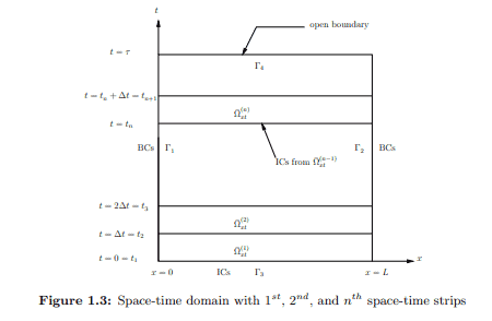
In space-time coupled methods for the whole space-time domain $\bar{\Omega}{x t}=$ $[0, L] \times[0, \tau]$, the computations can be intense and sometimes prohibitive if the final time $\tau$ is large. This problem can be easily overcome by using space-time strip or slab for an increment of time $\Delta t$ and then time-marching to obtain the entire evolution. Consider the space-time domain $$ \bar{\Omega}{x t}=\Omega_{x t} \cup \Gamma ; \quad \Gamma=\bigcup_{i=1}^{4} \Gamma_{i}
$$
shown in Fig. 1.3. For an increment of time $\Delta t$, that is for $0 \leq t \leq \Delta t$, consider the first space-time strip $\bar{\Omega}{x t}^{(1)}=[0, L] \times[0, \Delta t]$. If we are only interested in the evolution up to time $t=\Delta t$ and not beyond $t=\Delta t$, then the evolution in the space-time domain $[0, L] \times[\Delta t, \tau]$ has not taken place yet, hence does not influence the evolution for $\bar{\Omega}{x t}^{(1)}, t \in[0, \Delta t]$. We also note that for $\bar{\Omega}{x t}^{(1)}$, the boundary at $t=\Delta t$ is open boundary that is similar to the open boundary at $t=\tau$ for the whole space-time domain. We remark that BCs and ICs for $\bar{\Omega}{x t}$ and $\bar{\Omega}{x t}^{(1)}$ are identical in the sense of those that are known and those that are not known. For $\bar{\Omega}{x t}^{(2)}$, the second space-time strip, the BCs are the same as for $\bar{\Omega}{x t}^{(1)}$ but the ICs at $t=\Delta t$ are obtained from the computed evolution for $\bar{\Omega}{x t}^{(1)}$ at $t=\Delta t$. Now, with the known ICs at $t=\Delta t$, the second space-time strip $\bar{\Omega}{x t}^{(2)}$ is exactly similar to the first space-time strip $\bar{\Omega}{x t}^{(1)}$ in terms of BCs, ICs, and open boundary. For $\bar{\Omega}{x t}^{(1)}$, $t=\Delta t$ is open boundary whereas for $\bar{\Omega}{x t}^{(2)}, t=2 \Delta t$ is open boundary. Both open boundaries are at final values of time for the corresponding space-time strips.
In this process the evolution is computed for the first space-time strip $\bar{\Omega}{x t}^{(1)}=[0, L] \times[0, \Delta t]$ and refinements are carried out (in discretization and $p$ levels in the sense of finite element processes) until the evolution for $\bar{\Omega}{x t}^{(1)}$ is a converged solution. Using this converged solution for $\bar{\Omega}{x t}^{(1)}$, ICs are extracted at $t=\Delta t$ for $\bar{\Omega}{x t}^{(2)}$ and a converged evolution is computed for the second space-time strip $\bar{\Omega}_{x t}^{(2)}$. This process is continued until $t=\tau$ is reached.
数学代写|有限元方法代写Finite Element Method代考|Space-time decoupled or quasi methods
In space-time decoupled or quasi methods the solution $\phi=\phi(x, t)$ is assumed not to have simultaneous dependence on space coordinate $x$ and time $t$. Referring to the IVP (1.1) in spatial coordinate $x\left(\right.$ i.e. $\left.\mathbb{R}^{1}\right)$ and time $t$, the solution $\phi(x, t)$ is expressed as the product of two functions $g(x)$ and $h(t):$
$$
\phi(x, t)=g(x) h(t)
$$
where $g(x)$ is a known function that satisfies differentiability, continuity, and the completeness requirements (and others) as dictated by (1.1). We substitute (1.3) in (1.1) and obtain
$$
A(g(x) h(t))-f(x, t)=0 \quad \forall x, t \in \Omega_{x t}
$$
Integrating (1.4) over $\bar{\Omega}{x}=[0, L]$ while assuming $h(t)$ and its time derivatives to be constant for an instant of time, we can write $$ \int{\Omega_{x}}(A(g(x) h(t))-f(x, t)) d x=0
$$
Since $g(x)$ is known, the definite integral in (1.5) can be evaluated, thereby eliminating $g(x)$, its spatial derivatives (due to operator $A$ ), and more specifically spatial coordinate $x$ altogether. Hence, (1.5) reduces to
$$
A h(t)-\underset{\sim}{f}(t)=0 \quad \forall t \in(0, \tau)
$$
in which $A$ is a time differential operator and $f$ is only a function of time. In other words, (1.6) is an ordinary differential equation in time which can now be integrated using explicit or implicit time integration methods or finite element method in time to obtain $h(t) \forall t \in[0, \tau]$. Using this calculated $h(t)$ in (1.3), we now have the solution $\phi(x, t)$ :
$$
\phi(x, t)=g(x) h(t) \quad \forall x, t \in \bar{\Omega}_{x t}=[0, L] \times[0, \tau]
$$
有限元方法代考
数学代写|有限元方法代写Finite Element Method代考|Space-time coupled methods using space-time
在整个时空域的时空耦合方法中 $\bar{\Omega} x t=[0, L] \times[0, \tau]$ ,如果最后一次计算可能会很激烈,有时甚至令人望而却 步 $\tau$ 很大。这个问题可以很容易地通过使用时空带或平板来克服时间增量 $\Delta t$ 然后通过时间推进获得整个进化过 程。考虑时空域
$$
\bar{\Omega} x t=\Omega_{x t} \cup \Gamma ; \quad \Gamma=\bigcup_{i=1}^{4} \Gamma_{i}
$$
如图 $1.3$ 所示。对于时间增量 $\Delta t$, 那是为了 $0 \leq t \leq \Delta t$, 考虑第一个时空带 $\bar{\Omega} x t^{(1)}=[0, L] \times[0, \Delta t]$. 如果我 们只对时代的进化感兴趣 $t=\Delta t$ 并且不超过 $t=\Delta t$, 那么时空域的演化 $[0, L] \times[\Delta t, \tau]$ 还没有发生,因此不影 响进化 $\bar{\Omega} x t^{(1)}, t \in[0, \Delta t]$. 我们还注意到,对于 $\bar{\Omega} x t^{(1)}$ ,边界在 $t=\Delta t$ 是类似于开放边界的开放边界 $t=\tau$ 对 于整个时空域。我们注意到 $B C s$ 和 ICS 用于 $\bar{\Omega} x t$ 和 $\bar{\Omega} x t^{(1)}$ 在已知和末知的意义上是相同的。为了 $\bar{\Omega} x t^{(2)}$ ,第二 个时空带, $\mathrm{BC}$ 与 $\bar{\Omega} x t^{(1)}$ 但 $\mid$ 在 $t=\Delta t$ 从计算的进化中获得 $\bar{\Omega} x t^{(1)}$ 在 $t=\Delta t$. 现在,使用已知的 IC $t=\Delta t$ ,第 二个时空带 $\bar{\Omega} x t^{(2)}$ 与第一条时空条一模一样 $\bar{\Omega} x t^{(1)}$ 在 $B C 、 I C$ 和开放边界方面。为了 $\bar{\Omega} x t^{(1)}, t=\Delta t$ 是开放边 界,而对于 $\bar{\Omega} x t^{(2)}, t=2 \Delta t$ 是开放边界。对于相应的时空带,两个开放边界都处于最终时间值。
在这个过程中,计算第一个时空带的演化 $\bar{\Omega} x t^{(1)}=[0, L] \times[0, \Delta t]$ 并进行细化(离散化和 $p$ 有限元过程意义上 的水平) 直到进化 $\bar{\Omega} x t^{(1)}$ 是一个收敛的解决方案。使用此融合解决方案 $\bar{\Omega} x t^{(1)}$ ,IC 被提取在 $t=\Delta t$ 为了 $\bar{\Omega} x t^{(2)}$ 并计算第二个时空带的收敛演化 $\bar{\Omega}_{x t}^{(2)}$. 这个过程一直持续到 $t=\tau$ 到达了。
数学代写|有限元方法代写Finite Element Method代考|Space-time decoupled or quasi methods
在时空解耦或准方法中,解决方案 $\phi=\phi(x, t)$ 假定不同时依赖空间坐标 $x$ 和时间 $t$. 参考空间坐标中的IVP
$(1.1)$ $x\left(\mathbb{E} \mathbb{R}^{1}\right)$ 和时间 $t$ ,解决方案 $\phi(x, t)$ 表示为两个函数的乘积 $g(x)$ 和 $h(t)$ :
$$
\phi(x, t)=g(x) h(t)
$$
在哪里 $g(x)$ 是一个已知函数,它满足由 (1.1) 规定的可微性、连续性和完整性要求 (和其他要求) 。我们将 (1.3) 代入 (1.1) 并得到
$$
A(g(x) h(t))-f(x, t)=0 \quad \forall x, t \in \Omega_{x t}
$$
积分 (1.4) $\bar{\Omega} x=[0, L]$ 假设 $h(t)$ 并且它的时间导数在一瞬间是恒定的,我们可以写
$$
\int \Omega_{x}(A(g(x) h(t))-f(x, t)) d x=0
$$
自从 $g(x)$ 已知,可以计算 (1.5) 中的定积分,从而消除 $g(x)$ ,它的空间导数(由于算子 $A$ ),更具体地说是空间 坐标 $x$ 共。因此,(1.5) 简化为
$$
A h(t)-\underset{\sim}{f}(t)=0 \quad \forall t \in(0, \tau)
$$
其中 $A$ 是一个时间微分算子并且 $f$ 只是时间的函数。换句话说,(1.6) 是时间上的常微分方程,现在可以使用显式 或隐式时间积分方法或时间有限元方法积分得到 $h(t) \forall t \in[0, \tau]$. 使用这个计算 $h(t)$ 在 (1.3) 中,我们现在有了 解决方案 $\phi(x, t)$ :
$$
\phi(x, t)=g(x) h(t) \quad \forall x, t \in \bar{\Omega}_{x t}=[0, L] \times[0, \tau]
$$

统计代写请认准statistics-lab™. statistics-lab™为您的留学生涯保驾护航。
金融工程代写
金融工程是使用数学技术来解决金融问题。金融工程使用计算机科学、统计学、经济学和应用数学领域的工具和知识来解决当前的金融问题,以及设计新的和创新的金融产品。
非参数统计代写
非参数统计指的是一种统计方法,其中不假设数据来自于由少数参数决定的规定模型;这种模型的例子包括正态分布模型和线性回归模型。
广义线性模型代考
广义线性模型(GLM)归属统计学领域,是一种应用灵活的线性回归模型。该模型允许因变量的偏差分布有除了正态分布之外的其它分布。
术语 广义线性模型(GLM)通常是指给定连续和/或分类预测因素的连续响应变量的常规线性回归模型。它包括多元线性回归,以及方差分析和方差分析(仅含固定效应)。
有限元方法代写
有限元方法(FEM)是一种流行的方法,用于数值解决工程和数学建模中出现的微分方程。典型的问题领域包括结构分析、传热、流体流动、质量运输和电磁势等传统领域。
有限元是一种通用的数值方法,用于解决两个或三个空间变量的偏微分方程(即一些边界值问题)。为了解决一个问题,有限元将一个大系统细分为更小、更简单的部分,称为有限元。这是通过在空间维度上的特定空间离散化来实现的,它是通过构建对象的网格来实现的:用于求解的数值域,它有有限数量的点。边界值问题的有限元方法表述最终导致一个代数方程组。该方法在域上对未知函数进行逼近。[1] 然后将模拟这些有限元的简单方程组合成一个更大的方程系统,以模拟整个问题。然后,有限元通过变化微积分使相关的误差函数最小化来逼近一个解决方案。
tatistics-lab作为专业的留学生服务机构,多年来已为美国、英国、加拿大、澳洲等留学热门地的学生提供专业的学术服务,包括但不限于Essay代写,Assignment代写,Dissertation代写,Report代写,小组作业代写,Proposal代写,Paper代写,Presentation代写,计算机作业代写,论文修改和润色,网课代做,exam代考等等。写作范围涵盖高中,本科,研究生等海外留学全阶段,辐射金融,经济学,会计学,审计学,管理学等全球99%专业科目。写作团队既有专业英语母语作者,也有海外名校硕博留学生,每位写作老师都拥有过硬的语言能力,专业的学科背景和学术写作经验。我们承诺100%原创,100%专业,100%准时,100%满意。
随机分析代写
随机微积分是数学的一个分支,对随机过程进行操作。它允许为随机过程的积分定义一个关于随机过程的一致的积分理论。这个领域是由日本数学家伊藤清在第二次世界大战期间创建并开始的。
时间序列分析代写
随机过程,是依赖于参数的一组随机变量的全体,参数通常是时间。 随机变量是随机现象的数量表现,其时间序列是一组按照时间发生先后顺序进行排列的数据点序列。通常一组时间序列的时间间隔为一恒定值(如1秒,5分钟,12小时,7天,1年),因此时间序列可以作为离散时间数据进行分析处理。研究时间序列数据的意义在于现实中,往往需要研究某个事物其随时间发展变化的规律。这就需要通过研究该事物过去发展的历史记录,以得到其自身发展的规律。
回归分析代写
多元回归分析渐进(Multiple Regression Analysis Asymptotics)属于计量经济学领域,主要是一种数学上的统计分析方法,可以分析复杂情况下各影响因素的数学关系,在自然科学、社会和经济学等多个领域内应用广泛。
MATLAB代写
MATLAB 是一种用于技术计算的高性能语言。它将计算、可视化和编程集成在一个易于使用的环境中,其中问题和解决方案以熟悉的数学符号表示。典型用途包括:数学和计算算法开发建模、仿真和原型制作数据分析、探索和可视化科学和工程图形应用程序开发,包括图形用户界面构建MATLAB 是一个交互式系统,其基本数据元素是一个不需要维度的数组。这使您可以解决许多技术计算问题,尤其是那些具有矩阵和向量公式的问题,而只需用 C 或 Fortran 等标量非交互式语言编写程序所需的时间的一小部分。MATLAB 名称代表矩阵实验室。MATLAB 最初的编写目的是提供对由 LINPACK 和 EISPACK 项目开发的矩阵软件的轻松访问,这两个项目共同代表了矩阵计算软件的最新技术。MATLAB 经过多年的发展,得到了许多用户的投入。在大学环境中,它是数学、工程和科学入门和高级课程的标准教学工具。在工业领域,MATLAB 是高效研究、开发和分析的首选工具。MATLAB 具有一系列称为工具箱的特定于应用程序的解决方案。对于大多数 MATLAB 用户来说非常重要,工具箱允许您学习和应用专业技术。工具箱是 MATLAB 函数(M 文件)的综合集合,可扩展 MATLAB 环境以解决特定类别的问题。可用工具箱的领域包括信号处理、控制系统、神经网络、模糊逻辑、小波、仿真等。