如果你也在 怎样代写编码理论Coding Theory这个学科遇到相关的难题,请随时右上角联系我们的24/7代写客服。
编码理论是研究编码的属性和它们各自对特定应用的适用性。编码被用于数据压缩、密码学、错误检测和纠正、数据传输和数据存储。各种科学学科,如信息论、电气工程、数学、语言学和计算机科学,都对编码进行了研究,目的是设计高效和可靠的数据传输方法。这通常涉及消除冗余和纠正或检测传输数据中的错误。
statistics-lab™ 为您的留学生涯保驾护航 在代写编码理论Coding Theory方面已经树立了自己的口碑, 保证靠谱, 高质且原创的统计Statistics代写服务。我们的专家在代写编码理论Coding Theory代写方面经验极为丰富,各种代写编码理论Coding Theory相关的作业也就用不着说。
我们提供的编码理论Coding Theory及其相关学科的代写,服务范围广, 其中包括但不限于:
- Statistical Inference 统计推断
- Statistical Computing 统计计算
- Advanced Probability Theory 高等概率论
- Advanced Mathematical Statistics 高等数理统计学
- (Generalized) Linear Models 广义线性模型
- Statistical Machine Learning 统计机器学习
- Longitudinal Data Analysis 纵向数据分析
- Foundations of Data Science 数据科学基础
数学代写|编码理论作业代写Coding Theory代考|Code Parameters
Channel codes are characterised by so-called code parameters. The most important code parameters of a general $(n, k)$ block code that are introduced in the following are the code rate and the minimum Hamming distance (Bossert, 1999; Lin and Costello, 2004; Ling and Xing, 2004). With the help of these code parameters, the efficiency of the encoding process and the error detection and error correction capabilities can be evaluated for a given $(n, k)$ block code.
Code Rate
Under the assumption that each information symbol $u_{i}$ of the $(n, k)$ block code can assume $q$ values, the number of possible information words and code words is given by ${ }^{2}$
$$
M=q^{k} .
$$
Since the code word length $n$ is larger than the information word length $k$, the rate at which information is transmitted across the channel is reduced by the so-called code rate
$$
R=\frac{\log {q}(M)}{n}=\frac{k}{n} . $$ For the simple binary triple repetition code with $k=1$ and $n=3$, the code rate is $R=$ $\frac{k}{n}=\frac{1}{3} \approx 0,3333$. Weight and Hamming Distance Each code word $\mathbf{b}=\left(b{0}, b_{1}, \ldots, b_{n-1}\right)$ can be assigned the weight wt(b) which is defined as the number of non-zero components $b_{i} \neq 0$ (Bossert, 1999), i.e. ${ }^{3}$
$$
\operatorname{wt}(\mathbf{b})=\left|\left{i: b_{i} \neq 0,0 \leq i<n\right}\right| .
$$
Accordingly, the distance between two code words $\mathbf{b}=\left(b_{0}, b_{1}, \ldots, b_{n-1}\right)$ and $\mathbf{b}^{\prime}=\left(b_{0}^{\prime}\right.$, $\left.b_{1}^{\prime}, \ldots, b_{n-1}^{\prime}\right)$ is given by the so-called Hamming distance (Bossert, 1999)
$$
\operatorname{dist}\left(\mathbf{b}, \mathbf{b}^{\prime}\right)=\left|\left{i: b_{i} \neq b_{i}^{\prime}, 0 \leq i<n\right}\right| .
$$
The Hamming distance dist $\left(\mathbf{b}, \mathbf{b}^{\prime}\right)$ provides the number of different components of $\mathbf{b}$ and $\mathbf{b}^{\prime}$ and thus measures how close the code words $\mathbf{b}$ and $\mathbf{b}^{\prime}$ are to each other. For a code $\mathbb{B}$ consisting of $M$ code words $\mathbf{b}{1}, \mathbf{b}{2}, \ldots, \mathbf{b}{M}$, the minimum Hamming distance is given by $$ d=\min {\mathbf{b} \mathbf{b} \neq \mathbf{b}^{\prime}} \operatorname{dist}\left(\mathbf{b}, \mathbf{b}^{\prime}\right) .
$$
We will denote the $(n, k)$ block code $\mathrm{B}=\left{\mathbf{b}{1}, \mathbf{b}{2}, \ldots, \mathbf{b}{M}\right}$ with $M=q^{k} q$-nary code words of length $n$ and minimum Hamming distance $d$ by $\mathrm{B}(n, k, d)$. The minimum weight of the block code $\mathrm{B}$ is defined as $\min {\mathbf{b} \neq \mathbf{0}}$ wt(b). The code parameters of $\mathbb{B}(n, k, d)$ are summarised in Figure 2.4.
数学代写|编码理论作业代写Coding Theory代考|Maximum Likelihood Decoding
Channel codes are used in order to decrease the probability of incorrectly received code words or symbols. In this section we will derive a widely used decoding strategy. To this end, we will consider a decoding strategy to be optimal if the corresponding word error probability
$$
p_{\mathrm{err}}=\operatorname{Pr}{\hat{\mathbf{u}} \neq \mathbf{u}}=\operatorname{Pr}{\hat{\mathbf{b}} \neq \mathbf{b}}
$$
is minimal (Bossert, 1999). The word error probability has to be distinguished from the symbol error probability
$$
p_{\mathrm{sym}}=\frac{1}{k} \sum_{i=0}^{k-1} \operatorname{Pr}\left{\hat{u}{i} \neq u{i}\right}
$$
which denotes the probability of an incorrectly decoded information symbol $u_{i}$. In general, the symbol error probability is harder to derive analytically than the word error probability. However, it can be bounded by the following inequality (Bossert, 1999)
$$
\frac{1}{k} p_{\mathrm{err}} \leq p_{\mathrm{sym}} \leq p_{\mathrm{err}} .
$$
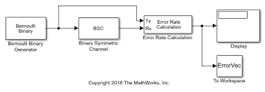
In the following, a $q$-nary channel code $\mathrm{B} \in \mathrm{F}{q}^{n}$ with $M$ code words $\mathbf{b}{1}, \mathbf{b}{2}, \ldots, \mathbf{b}{M}$ in the code space $\mathrm{F}{q}^{n}$ is considered. Let $\mathbf{b}{j}$ be the transmitted code word. Owing to the noisy channel, the received word $\mathbf{r}$ may differ from the transmitted code word $\mathbf{b}{j}$. The task of the decoder in Figure $2.6$ is to decode the transmitted code word based on the sole knowledge of $\mathbf{r}$ with minimal word error probability $p{\text {err }}$.
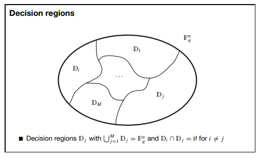
This decoding step can be written according to the decoding rule $\mathbf{r} \mapsto \hat{\mathbf{b}}=\hat{\mathbf{b}}(\mathbf{r})$. For hard-decision decoding the received word $\mathbf{r}$ is an element of the discrete code space $\mathbb{F}{q}^{n}$. To each code word $\mathbf{b}{j}$ we assign a corresponding subspace $\mathrm{D}{j}$ of the code space $\mathbb{F}{q}^{n}$, the so-called decision region. These non-overlapping decision regions create the whole code space $\mathbb{F}{q}^{n}$, i.e. $\bigcup{j=1}^{M} \mathbb{D}{j}=\mathbb{F}{q}^{n}$ and $\mathbb{D}{i} \cap \mathbb{D}{j}=\emptyset$ for $i \neq j$ as illustrated in Figure 2.7. If the received word $\mathbf{r}$ lies within the decision region $\mathbb{D}{i}$, the decoder decides in favour of the code word $\mathbf{b}{i}$. That is, the decoding of the code word $\mathbf{b}{i}$ according to the decision rule $\hat{\mathbf{b}}(\mathbf{r})=\mathbf{b}{i}$ is equivalent to the event $\mathbf{r} \in \mathbb{D}{i}$. By properly choosing the decision regions $\mathbb{D}{i}$, the decoder can be designed. For an optimal decoder the decision regions are chosen such that the word error probability $p_{\mathrm{err}}$ is minimal.
The probability of the event that the code word $\mathbf{b}=\mathbf{b}{j}$ is transmitted and the code word $\hat{\mathbf{b}}(\mathbf{r})=\mathbf{b}{i}$ is decoded is given by
$$
\operatorname{Pr}\left{\left(\hat{\mathbf{b}}(\mathbf{r})=\mathbf{b}{i}\right) \wedge\left(\mathbf{b}=\mathbf{b}{j}\right)\right}=\operatorname{Pr}\left{\left(\mathbf{r} \in \mathbb{D}{i}\right) \wedge\left(\mathbf{b}=\mathbf{b}{j}\right)\right} .
$$
We obtain the word error probability $p_{\text {err }}$ by averaging over all possible events for which the transmitted code word $\mathbf{b}=\mathbf{b}{j}$ is decoded into a different code word $\hat{\mathbf{b}}(\mathbf{r})=\mathbf{b}{i}$ with
$i \neq j$. This leads to (Neubauer, 2006b)
$$
\begin{aligned}
p_{\mathrm{err}} &=\operatorname{Pr}{\hat{\mathbf{b}}(\mathbf{r}) \neq \mathbf{b}} \
&=\sum_{i=1}^{M} \sum_{j \neq i} \operatorname{Pr}\left{\left(\hat{\mathbf{b}}(\mathbf{r})=\mathbf{b}{i}\right) \wedge\left(\mathbf{b}=\mathbf{b}{j}\right)\right} \
&=\sum_{i=1}^{M} \sum_{j \neq i} \operatorname{Pr}\left{\left(\mathbf{r} \in \mathbb{D}{i}\right) \wedge\left(\mathbf{b}=\mathbf{b}{j}\right)\right} \
&=\sum_{i=1}^{M} \sum_{j \neq i} \sum_{\mathbf{r} \in \mathrm{D}{i}} \operatorname{Pr}\left{\mathbf{r} \wedge\left(\mathbf{b}=\mathbf{b}{j}\right)\right}
\end{aligned}
$$
With the help of Bayes’ rule $\operatorname{Pr}\left{\mathbf{r} \wedge\left(\mathbf{b}=\mathbf{b}{j}\right)\right}=\operatorname{Pr}\left{\mathbf{b}=\mathbf{b}{j} \mid \mathbf{r}\right} \operatorname{Pr}{\mathbf{r}}$ and by changing the order of summation, we obtain
$$
\begin{aligned}
p_{e r r} &=\sum_{i=1}^{M} \sum_{\mathbf{r} \in \mathrm{D}{i}} \sum{j \neq i} \operatorname{Pr}\left{\mathbf{r} \wedge\left(\mathbf{b}=\mathbf{b}{j}\right)\right} \ &=\sum{i=1}^{M} \sum_{\mathbf{r} \in \mathrm{D}{i}} \sum{j \neq i} \operatorname{Pr}\left{\mathbf{b}=\mathbf{b}_{j} \mid \mathbf{r}\right} \operatorname{Pr}{\mathbf{r}}
\end{aligned}
$$
数学代写|编码理论作业代写Coding Theory代考|Binary Symmetric Channel
In Section $1.2 .3$ we defined the binary symmetric channel as a memoryless channel with the conditional probabilities
$$
\operatorname{Pr}\left{r_{i} \mid b_{i}\right}=\left{\begin{array}{cc}
1-\varepsilon, & r_{i}=b_{i} \
\varepsilon, & r_{i} \neq b_{i}
\end{array}\right.
$$
with channel bit error probability $\varepsilon$. Since the binary symmetric channel is assumed to be memoryless, the conditional probability $\operatorname{Pr}{\mathbf{r} \mid \mathbf{b}}$ can be calculated for code word $\mathbf{b}=$
$\left(b_{0}, b_{1}, \ldots, b_{n-1}\right)$ and received word $\mathbf{r}=\left(r_{0}, r_{1}, \ldots, r_{n-1}\right)$ according to
$$
\operatorname{Pr}{\mathbf{r} \mid \mathbf{b}}=\prod_{i=0}^{n-1} \operatorname{Pr}\left{r_{i} \mid b_{i}\right}
$$
If the words $\mathbf{r}$ and $\mathbf{b}$ differ in $\operatorname{dist}(\mathbf{r}, \mathbf{b})$ symbols, this yields
$$
\operatorname{Pr}{\mathbf{r} \mid \mathbf{b}}=(1-\varepsilon)^{n-\operatorname{dist}(\mathbf{r}, \mathbf{b})} \varepsilon^{\operatorname{dist}(\mathbf{r}, \mathbf{b})}=(1-\varepsilon)^{n}\left(\frac{\varepsilon}{1-\varepsilon}\right)^{\operatorname{dist}(\mathbf{r}, \mathbf{b})}
$$
Taking into account $0 \leq \varepsilon<\frac{1}{2}$ and therefore $\frac{\varepsilon}{1-\varepsilon}<1$, the MLD rule is given by
$$
\hat{\mathbf{b}}(\mathbf{r})=\underset{\mathbf{b} \in \mathrm{B}}{\operatorname{argmax}} \operatorname{Pr}{\mathbf{r} \mid \mathbf{b}}=\underset{\mathbf{b} \in \mathrm{B}}{\operatorname{argmax}}(1-\varepsilon)^{n}\left(\frac{\varepsilon}{1-\varepsilon}\right)^{\operatorname{dist}(\mathbf{r}, \mathbf{b})}=\underset{\mathbf{b} \in \mathrm{B}}{\operatorname{argmin}} \operatorname{dist}(\mathbf{r}, \mathbf{b}),
$$
i.e. for the binary symmetric channel the optimal maximum likelihood decoder (Bossert, 1999)
$$
\hat{\mathbf{b}}(\mathbf{r})=\underset{\mathbf{b} \in \mathbb{B}}{\operatorname{argmin}} \operatorname{dist}(\mathbf{r}, \mathbf{b})
$$
emits that particular code word which differs in the smallest number of components from the received word $\mathbf{r}$, i.e. which has the smallest Hamming distance to the received word $\mathbf{r}$ (see Figure 2.9). This decoding rule is called minimum distance decoding. This minimum distance decoding rule is also optimal for a $q$-nary symmetric channel (Neubauer, 2006b). We now turn to the error probabilities for the binary symmetric channel during transmission before decoding. The probability of $w$ errors at $w$ given positions within the $n$-dimensional binary received word $\mathbf{r}$ is given by $\varepsilon^{w}(1-\varepsilon)^{n-w}$. Since there are $\left(\begin{array}{l}n \ w\end{array}\right)$ different possibilities
of choosing $w$ out of $n$ positions, the probability of $w$ errors at arbitrary positions within an $n$-dimensional binary received word follows the binomial distribution
$$
\operatorname{Pr}{w \text { errors }}=\left(\begin{array}{c}
n \
w
\end{array}\right) \varepsilon^{w}(1-\varepsilon)^{n-w}
$$
with mean $n \varepsilon$. Because of the condition $\varepsilon<\frac{1}{2}$, the probability $\operatorname{Pr}{w$ errors $}$ decreases with increasing number of errors $w$, i.e. few errors are more likely than many errors.
The probability of error-free transmission is $\operatorname{Pr}{0$ errors $}=(1-\varepsilon)^{n}$, whereas the probability of a disturbed transmission with $\mathbf{r} \neq \mathbf{b}$ is given by
$$
\operatorname{Pr}{\mathbf{r} \neq \mathbf{b}}=\sum_{w=1}^{n}\left(\begin{array}{l}
n \
w
\end{array}\right) \varepsilon^{w}(1-\varepsilon)^{n-w}=1-(1-\varepsilon)^{n} .
$$
编码理论代写
数学代写|编码理论作业代写Coding Theory代考|Code Parameters
信道代码的特征在于所谓的代码参数。一般最重要的代码参数(n,ķ)下面介绍的块码是码率和最小汉明距离(Bossert,1999;Lin 和 Costello,2004;Ling 和 Xing,2004)。借助这些代码参数,可以评估给定编码过程的效率以及错误检测和纠错能力(n,ķ)块代码。
码率
假设每个信息符号在一世的(n,ķ)块代码可以假设q值,可能的信息字和代码字的数量由下式给出2
米=qķ.
由于码字长n大于信息字长ķ,通过信道传输信息的速率被所谓的码率降低
R=日志q(米)n=ķn.对于简单的二进制三重重复代码ķ=1和n=3,码率为R= ķn=13≈0,3333. 权重和汉明距离每个码字b=(b0,b1,…,bn−1)可以分配权重 wt(b),定义为非零分量的数量b一世≠0(博塞特,1999),即3
\operatorname{wt}(\mathbf{b})=\left|\left{i: b_{i} \neq 0,0 \leq i<n\right}\right| .\operatorname{wt}(\mathbf{b})=\left|\left{i: b_{i} \neq 0,0 \leq i<n\right}\right| .
因此,两个码字之间的距离b=(b0,b1,…,bn−1)和b′=(b0′, b1′,…,bn−1′)由所谓的汉明距离给出 (Bossert, 1999)
\operatorname{dist}\left(\mathbf{b}, \mathbf{b}^{\prime}\right)=\left|\left{i: b_{i} \neq b_{i}^{\prime }, 0 \leq i<n\right}\right| .\operatorname{dist}\left(\mathbf{b}, \mathbf{b}^{\prime}\right)=\left|\left{i: b_{i} \neq b_{i}^{\prime }, 0 \leq i<n\right}\right| .
汉明距离 dist(b,b′)提供不同组件的数量b和b′从而测量代码字的接近程度b和b′是彼此的。对于一个代码乙包含由…组成米暗语b1,b2,…,b米,最小汉明距离由下式给出
d=分钟bb≠b′距离(b,b′).
我们将表示(n,ķ)块代码\mathrm{B}=\left{\mathbf{b}{1}, \mathbf{b}{2}, \ldots, \mathbf{b}{M}\right}\mathrm{B}=\left{\mathbf{b}{1}, \mathbf{b}{2}, \ldots, \mathbf{b}{M}\right}和米=qķq-nary码字长度n和最小汉明距离d经过乙(n,ķ,d). 块码的最小权重乙定义为分钟b≠0重量(b)。代码参数乙(n,ķ,d)总结在图 2.4 中。
数学代写|编码理论作业代写Coding Theory代考|Maximum Likelihood Decoding
使用信道代码是为了降低错误接收代码字或符号的概率。在本节中,我们将推导出一种广泛使用的解码策略。为此,我们将考虑一个解码策略是最优的,如果相应的单词错误概率
p和rr=公关在^≠在=公关b^≠b
是最小的(Bossert,1999)。字错误概率必须与符号错误概率区分开来
p_{\mathrm{sym}}=\frac{1}{k} \sum_{i=0}^{k-1} \operatorname{Pr}\left{\hat{u}{i} \neq u{我}\右}p_{\mathrm{sym}}=\frac{1}{k} \sum_{i=0}^{k-1} \operatorname{Pr}\left{\hat{u}{i} \neq u{我}\右}
表示错误解码的信息符号的概率在一世. 一般来说,符号错误概率比字错误概率更难解析推导。然而,它可以受到以下不等式的限制(Bossert,1999)
1ķp和rr≤ps是米≤p和rr.
在下文中,一个q-nary 频道代码乙∈Fqn和米暗语b1,b2,…,b米在代码空间Fqn被认为。让bj是传输的码字。由于信道嘈杂,接收到的词r可能与传输的代码字不同bj. 图中解码器的任务2.6是根据唯一的知识对传输的码字进行解码r具有最小的单词错误概率p呃 .
这个解码步骤可以根据解码规则来写r↦b^=b^(r). 对于接收到的字进行硬决策解码r是离散码空间的一个元素Fqn. 对每个码字bj我们分配一个相应的子空间Dj代码空间Fqn,即所谓的决策区域。这些不重叠的决策区域创建了整个代码空间Fqn, IE⋃j=1米Dj=Fqn和D一世∩Dj=∅为了一世≠j如图 2.7 所示。如果收到的话r位于决策区域内D一世,解码器决定支持码字b一世. 也就是码字的解码b一世根据决策规则b^(r)=b一世相当于事件r∈D一世. 通过正确选择决策区域D一世,可以设计解码器。对于最佳解码器,选择决策区域使得单词错误概率p和rr是最小的。
码字发生事件的概率b=bj被传输和代码字b^(r)=b一世被解码由下式给出
\operatorname{Pr}\left{\left(\hat{\mathbf{b}}(\mathbf{r})=\mathbf{b}{i}\right) \wedge\left(\mathbf{b}= \mathbf{b}{j}\right)\right}=\operatorname{Pr}\left{\left(\mathbf{r} \in \mathbb{D}{i}\right) \wedge\left(\ mathbf{b}=\mathbf{b}{j}\right)\right} 。\operatorname{Pr}\left{\left(\hat{\mathbf{b}}(\mathbf{r})=\mathbf{b}{i}\right) \wedge\left(\mathbf{b}= \mathbf{b}{j}\right)\right}=\operatorname{Pr}\left{\left(\mathbf{r} \in \mathbb{D}{i}\right) \wedge\left(\ mathbf{b}=\mathbf{b}{j}\right)\right} 。
我们得到单词错误概率p呃 通过对传输代码字的所有可能事件进行平均b=bj被解码成不同的码字b^(r)=b一世和
一世≠j. 这导致(纽鲍尔,2006b)
\begin{aligned} p_{\mathrm{err}} &=\operatorname{Pr}{\hat{\mathbf{b}}(\mathbf{r}) \neq \mathbf{b}} \ &=\sum_ {i=1}^{M} \sum_{j \neq i} \operatorname{Pr}\left{\left(\hat{\mathbf{b}}(\mathbf{r})=\mathbf{b} {i}\right) \wedge\left(\mathbf{b}=\mathbf{b}{j}\right)\right} \ &=\sum_{i=1}^{M} \sum_{j \ neq i} \operatorname{Pr}\left{\left(\mathbf{r} \in \mathbb{D}{i}\right) \wedge\left(\mathbf{b}=\mathbf{b}{j }\right)\right} \ &=\sum_{i=1}^{M} \sum_{j \neq i} \sum_{\mathbf{r} \in \mathrm{D}{i}} \operatorname {Pr}\left{\mathbf{r} \wedge\left(\mathbf{b}=\mathbf{b}{j}\right)\right} \end{对齐}\begin{aligned} p_{\mathrm{err}} &=\operatorname{Pr}{\hat{\mathbf{b}}(\mathbf{r}) \neq \mathbf{b}} \ &=\sum_ {i=1}^{M} \sum_{j \neq i} \operatorname{Pr}\left{\left(\hat{\mathbf{b}}(\mathbf{r})=\mathbf{b} {i}\right) \wedge\left(\mathbf{b}=\mathbf{b}{j}\right)\right} \ &=\sum_{i=1}^{M} \sum_{j \ neq i} \operatorname{Pr}\left{\left(\mathbf{r} \in \mathbb{D}{i}\right) \wedge\left(\mathbf{b}=\mathbf{b}{j }\right)\right} \ &=\sum_{i=1}^{M} \sum_{j \neq i} \sum_{\mathbf{r} \in \mathrm{D}{i}} \operatorname {Pr}\left{\mathbf{r} \wedge\left(\mathbf{b}=\mathbf{b}{j}\right)\right} \end{对齐}
借助贝叶斯法则\operatorname{Pr}\left{\mathbf{r} \wedge\left(\mathbf{b}=\mathbf{b}{j}\right)\right}=\operatorname{Pr}\left{\mathbf{ b}=\mathbf{b}{j} \mid \mathbf{r}\right} \operatorname{Pr}{\mathbf{r}}\operatorname{Pr}\left{\mathbf{r} \wedge\left(\mathbf{b}=\mathbf{b}{j}\right)\right}=\operatorname{Pr}\left{\mathbf{ b}=\mathbf{b}{j} \mid \mathbf{r}\right} \operatorname{Pr}{\mathbf{r}}并且通过改变求和的顺序,我们得到
\begin{对齐} p_{e r r} &=\sum_{i=1}^{M} \sum_{\mathbf{r} \in \mathrm{D}{i}} \sum{j \neq i} \运算符名{Pr}\left{\mathbf{r} \wedge\left(\mathbf{b}=\mathbf{b}{j}\right)\right} \ &=\sum{i=1}^{M } \sum_{\mathbf{r} \in \mathrm{D}{i}} \sum{j \neq i} \operatorname{Pr}\left{\mathbf{b}=\mathbf{b}_{j } \mid \mathbf{r}\right} \operatorname{Pr}{\mathbf{r}} \end{aligned}\begin{对齐} p_{e r r} &=\sum_{i=1}^{M} \sum_{\mathbf{r} \in \mathrm{D}{i}} \sum{j \neq i} \运算符名{Pr}\left{\mathbf{r} \wedge\left(\mathbf{b}=\mathbf{b}{j}\right)\right} \ &=\sum{i=1}^{M } \sum_{\mathbf{r} \in \mathrm{D}{i}} \sum{j \neq i} \operatorname{Pr}\left{\mathbf{b}=\mathbf{b}_{j } \mid \mathbf{r}\right} \operatorname{Pr}{\mathbf{r}} \end{aligned}
数学代写|编码理论作业代写Coding Theory代考|Binary Symmetric Channel
在部分1.2.3我们将二进制对称通道定义为无记忆通道,条件概率为
$$
\operatorname{Pr}\left{r_{i} \mid b_{i}\right}=\left{
1−e,r一世=b一世 e,r一世≠b一世\正确的。
$$
与信道误码概率e. 由于假设二进制对称信道是无记忆的,因此条件概率公关r∣b可以计算码字b=
(b0,b1,…,bn−1)并收到消息r=(r0,r1,…,rn−1)根据
\operatorname{Pr}{\mathbf{r} \mid \mathbf{b}}=\prod_{i=0}^{n-1} \operatorname{Pr}\left{r_{i} \mid b_{i }\正确的}\operatorname{Pr}{\mathbf{r} \mid \mathbf{b}}=\prod_{i=0}^{n-1} \operatorname{Pr}\left{r_{i} \mid b_{i }\正确的}
如果的话r和b不同之处距离(r,b)符号,这会产生
公关r∣b=(1−e)n−距离(r,b)e距离(r,b)=(1−e)n(e1−e)距离(r,b)
考虑在内0≤e<12因此e1−e<1, MLD 规则由下式给出
b^(r)=最大参数b∈乙公关r∣b=最大参数b∈乙(1−e)n(e1−e)距离(r,b)=精氨酸b∈乙距离(r,b),
即对于二进制对称信道,最佳最大似然解码器(Bossert,1999)
b^(r)=精氨酸b∈乙距离(r,b)
发出特定的代码字,该代码字与接收到的字的分量数量最少r,即与接收到的词的汉明距离最小r(见图 2.9)。这种解码规则称为最小距离解码。这个最小距离解码规则对于q-nary 对称通道(Neubauer,2006b)。我们现在转向在解码之前传输期间二进制对称信道的错误概率。的概率在错误在在在给定的位置n维二进制接收字r是(谁)给的e在(1−e)n−在. 既然有(n 在)不同的可能性
的选择在在……之外n位置,概率在内任意位置的误差n维二进制接收字服从二项分布
公关在 错误 =(n 在)e在(1−e)n−在
平均ne. 因为条件e<12, 概率公关在$和rr这rs$随着错误数量的增加而减少在,即少数错误比很多错误更可能发生。
无差错传输的概率为公关0$和rr这rs$=(1−e)n,而干扰传输的概率与r≠b是(谁)给的
公关r≠b=∑在=1n(n 在)e在(1−e)n−在=1−(1−e)n.

统计代写请认准statistics-lab™. statistics-lab™为您的留学生涯保驾护航。
金融工程代写
金融工程是使用数学技术来解决金融问题。金融工程使用计算机科学、统计学、经济学和应用数学领域的工具和知识来解决当前的金融问题,以及设计新的和创新的金融产品。
非参数统计代写
非参数统计指的是一种统计方法,其中不假设数据来自于由少数参数决定的规定模型;这种模型的例子包括正态分布模型和线性回归模型。
广义线性模型代考
广义线性模型(GLM)归属统计学领域,是一种应用灵活的线性回归模型。该模型允许因变量的偏差分布有除了正态分布之外的其它分布。
术语 广义线性模型(GLM)通常是指给定连续和/或分类预测因素的连续响应变量的常规线性回归模型。它包括多元线性回归,以及方差分析和方差分析(仅含固定效应)。
有限元方法代写
有限元方法(FEM)是一种流行的方法,用于数值解决工程和数学建模中出现的微分方程。典型的问题领域包括结构分析、传热、流体流动、质量运输和电磁势等传统领域。
有限元是一种通用的数值方法,用于解决两个或三个空间变量的偏微分方程(即一些边界值问题)。为了解决一个问题,有限元将一个大系统细分为更小、更简单的部分,称为有限元。这是通过在空间维度上的特定空间离散化来实现的,它是通过构建对象的网格来实现的:用于求解的数值域,它有有限数量的点。边界值问题的有限元方法表述最终导致一个代数方程组。该方法在域上对未知函数进行逼近。[1] 然后将模拟这些有限元的简单方程组合成一个更大的方程系统,以模拟整个问题。然后,有限元通过变化微积分使相关的误差函数最小化来逼近一个解决方案。
tatistics-lab作为专业的留学生服务机构,多年来已为美国、英国、加拿大、澳洲等留学热门地的学生提供专业的学术服务,包括但不限于Essay代写,Assignment代写,Dissertation代写,Report代写,小组作业代写,Proposal代写,Paper代写,Presentation代写,计算机作业代写,论文修改和润色,网课代做,exam代考等等。写作范围涵盖高中,本科,研究生等海外留学全阶段,辐射金融,经济学,会计学,审计学,管理学等全球99%专业科目。写作团队既有专业英语母语作者,也有海外名校硕博留学生,每位写作老师都拥有过硬的语言能力,专业的学科背景和学术写作经验。我们承诺100%原创,100%专业,100%准时,100%满意。
随机分析代写
随机微积分是数学的一个分支,对随机过程进行操作。它允许为随机过程的积分定义一个关于随机过程的一致的积分理论。这个领域是由日本数学家伊藤清在第二次世界大战期间创建并开始的。
时间序列分析代写
随机过程,是依赖于参数的一组随机变量的全体,参数通常是时间。 随机变量是随机现象的数量表现,其时间序列是一组按照时间发生先后顺序进行排列的数据点序列。通常一组时间序列的时间间隔为一恒定值(如1秒,5分钟,12小时,7天,1年),因此时间序列可以作为离散时间数据进行分析处理。研究时间序列数据的意义在于现实中,往往需要研究某个事物其随时间发展变化的规律。这就需要通过研究该事物过去发展的历史记录,以得到其自身发展的规律。
回归分析代写
多元回归分析渐进(Multiple Regression Analysis Asymptotics)属于计量经济学领域,主要是一种数学上的统计分析方法,可以分析复杂情况下各影响因素的数学关系,在自然科学、社会和经济学等多个领域内应用广泛。
MATLAB代写
MATLAB 是一种用于技术计算的高性能语言。它将计算、可视化和编程集成在一个易于使用的环境中,其中问题和解决方案以熟悉的数学符号表示。典型用途包括:数学和计算算法开发建模、仿真和原型制作数据分析、探索和可视化科学和工程图形应用程序开发,包括图形用户界面构建MATLAB 是一个交互式系统,其基本数据元素是一个不需要维度的数组。这使您可以解决许多技术计算问题,尤其是那些具有矩阵和向量公式的问题,而只需用 C 或 Fortran 等标量非交互式语言编写程序所需的时间的一小部分。MATLAB 名称代表矩阵实验室。MATLAB 最初的编写目的是提供对由 LINPACK 和 EISPACK 项目开发的矩阵软件的轻松访问,这两个项目共同代表了矩阵计算软件的最新技术。MATLAB 经过多年的发展,得到了许多用户的投入。在大学环境中,它是数学、工程和科学入门和高级课程的标准教学工具。在工业领域,MATLAB 是高效研究、开发和分析的首选工具。MATLAB 具有一系列称为工具箱的特定于应用程序的解决方案。对于大多数 MATLAB 用户来说非常重要,工具箱允许您学习和应用专业技术。工具箱是 MATLAB 函数(M 文件)的综合集合,可扩展 MATLAB 环境以解决特定类别的问题。可用工具箱的领域包括信号处理、控制系统、神经网络、模糊逻辑、小波、仿真等。