如果你也在 怎样代写计算复杂度理论Computational complexity theory这个学科遇到相关的难题,请随时右上角联系我们的24/7代写客服。
计算复杂度理论的重点是根据资源使用情况对计算问题进行分类,并将这些类别相互联系起来。计算问题是一项由计算机解决的任务。一个计算问题是可以通过机械地应用数学步骤来解决的,比如一个算法。
statistics-lab™ 为您的留学生涯保驾护航 在代写计算复杂度理论Computational complexity theory方面已经树立了自己的口碑, 保证靠谱, 高质且原创的统计Statistics代写服务。我们的专家在代写计算复杂度理论Computational complexity theory代写方面经验极为丰富,各种代写计算复杂度理论Computational complexity theory相关的作业也就用不着说。
我们提供的计算复杂度理论Computational complexity theory及其相关学科的代写,服务范围广, 其中包括但不限于:
- Statistical Inference 统计推断
- Statistical Computing 统计计算
- Advanced Probability Theory 高等概率论
- Advanced Mathematical Statistics 高等数理统计学
- (Generalized) Linear Models 广义线性模型
- Statistical Machine Learning 统计机器学习
- Longitudinal Data Analysis 纵向数据分析
- Foundations of Data Science 数据科学基础
数学代写|计算复杂度理论代写Computational complexity theory代考|Complex Networks: A Very Short Overview
Nowadays, Complex Networks represent a vibrant and independent research field that attracted the attention of scientists coming from different areas. The underlying reason is that many natural and man-made complex systems, as biological neural networks, social networks, and infrastructural networks, have a nontrivial topology that strongly influences the dynamics among the related agents (i.e., users of social networks, neurons of neural networks, and so on). An increasing amount of
investigations is demonstrating the relevance of the interaction structure in a wide amount of systems, and, even in the case of EGT, complex networks allow to obtain very interesting results. For instance, as recalled in Chap. 1, Santos and Pacheco showed the role of heterogeneity in the emergence of cooperation, modeling their system with scale-free networks. The latter, as well as others famous models, often is used as toy model both in EGT and in many other contexts as social dynamics, ecological networks, etc. Thus, in this section, we provide a very short overview on the main network properties, and on three different models that can be used for generating a complex network with a known topology. Readers interested in this topic are warmly encouraged to read the wide literature on complex networks. So, first of all, modern network theory has its basis in the classical theory of graphs. In particular, a preliminary definition of complex network can be “a graph with a nontrivial topology.” In general, a graph is a mathematical object that allows to represent relations among a collection of items, named nodes. More formally, a graph $G$ is defined as $G=(N, E)$, with $N$ set of nodes/vertices and $E$ set of edges/links (or bonds). Nodes can be described by a label and represent the elements of a system, e.g., users of a social network, websites of the WEB, and so on. In turn, the edges represent the connections among nodes, and map relations as friendship, physical links, etc. A graph can be “directed” or “undirected,” i.e., the relation can be symmetrical (e.g., friendship) or not (e.g., a one way road), and can be “weighted” or “unweighted.” The former allows to introduce some coarseness in the relations, e.g., in a transportation network the weights might refer to the actual geographical distance between two locations. The information related to the connections in a network is saved in a $N \times N$ matrix, with $N$ number of nodes, defined “adjacency matrix.” Numerical analysis on the adjacency matrix allow to investigate the properties of a network. For instance, the adjacency matrix $A$ of an unweighted graph can have the following form:
$$
a_{i j}= \begin{cases}1 & \text { if } e_{i j} \text { is defined } \ 0 & \text { if } e_{i j} \text { is not defined }\end{cases}
$$
On the other hand, in the case of weighted networks, the inner values of the adjacency matrix are real. Among the properties of a complex network, the degree distribution is one of the most relevant. Notably, this “centrality measure” constitutes a kind of signature for classifying the nature of a network (e.g., scalefree), where the term “degree” means amount of connections (i.e., edges) of a node. So, indicating with $k$ the degree of nodes, the distribution $P(k)$ of a network represents the probability to randomly select a node with a degree equal to $k$, i.e., a node with $k$ connections. A second network property is called clustering coefficient, and it allows to know if nodes of a network tend to cluster together. Actually, this phenomenon is common in many real networks as social networks, where it is possible to identify circles of friends, or acquaintances in which every person knows all the others. For the sake of clarity, considering a social network, if the user
$a$ is connected to the user $b$, and the latter is connected to the user $c$, there is a high probability that $a$ be connected to $c$. The clustering coefficient can be computed as
$$
C=\frac{3 \times T n}{T p}
$$
with $T n$ number of triangles in a network, and $T p$ number of connected triples of nodes. A connected triple is a single node with links running to an unordered pair of others. This coefficient has a range that spans the interval $0 \leq C \leq 1$. A further mathematical definition of the clustering coefficient reads
$$
C_{i}=\frac{T n_{i}}{T p_{i}}
$$
with $T n_{i}$ number of triangles connected to node $i$, and $T p_{i}$ number of triples centered on node $i$. The main difference between the two definitions is that the second one is local, so that to obtain a global value one has to compute the following parameter
$$
C=\frac{1}{n} \sum_{i} C_{i}
$$
数学代写|计算复杂度理论代写Computational complexity theory代考|Classical Random Networks
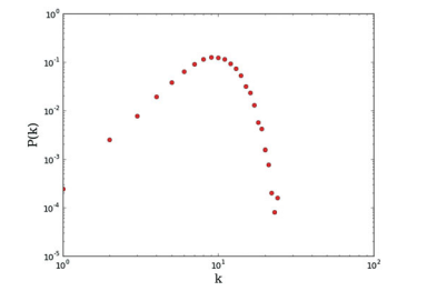
One of the early works on random networks has been developed by Paul Erdös and Alfred Renyi. Their model, usually called E-R model/graph, considers a graph with $N$ nodes and a probability $p$ to generate each edge. Accordingly, an E-R graph contains about $p \cdot \frac{N(N-1)}{2}$ edges, and it has a binomial degree distribution
$$
P(k)=\left(\begin{array}{c}
N-1 \
k
\end{array}\right) p^{k}(1-p)^{n-1-k}
$$
for $N \rightarrow$ inf and $n p=$ const, the degree distribution converges to a Poissonian distribution
$$
P(k) \sim e^{-p n} \cdot \frac{(p n)^{k}}{k !}
$$
To generate this kind of networks, one can implement the following simple algorithm:
- Define the number of $N$ of nodes and the probability $p$ for each edge
- Draw each potential-link with probability $p$
Figure $2.4$ illustrates the $P(k)$ for an E-R graph with $N=25,000$ and $p=4 \cdot 10^{-4}$.
数学代写|计算复杂度理论代写Computational complexity theory代考|Scale-Free Networks
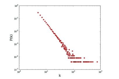
Scale-free networks are characterized by the presence of few nodes (called hubs) that have many connections (i.e., a high degree), while the majority of nodes has a low degree. Therefore, these networks constitute a classical example of heterogeneous networks. The related degree distribution follows a power-law function
$$
P(k) \sim c \cdot k^{-\gamma}
$$
with $c$ normalizing constant and $\gamma$ scaling parameter of the distribution. A famous model for generating scale-free networks is the Barabasi-Albert model (BA model hereinafter) that considers two parameters: $N$ nodes and $m$ minimum number of edges drawn for each node. The BA model can be summarized as follows:
- Define $N$ number of nodes and $m$ minimum number of edges drawn for each node
- Add a new node and link it with other $m$ pre-existing nodes. Pre-existing nodes are selected according to the following equation:
$$
\Pi\left(k_{i}\right)=\frac{k_{i}}{\sum_{j} k_{j}}
$$
with $\Pi\left(k_{i}\right)$ probability that the new node generates a link with the $i$-th node (having a $k_{i}$ degree).
Figure $2.5$ illustrates the $P(k)$ for a scale-free network with $N=25,000$ and $m=5$.
计算复杂度理论代考
数学代写|计算复杂度理论代写Computational complexity theory代考|Complex Networks: A Very Short Overview
如今,复杂网络代表了一个充满活力和独立的研究领域,吸引了来自不同领域的科学家的关注。根本原因是许多自然和人造的复杂系统,如生物神经网络、社交网络和基础设施网络,都有一个非平凡的拓扑结构,它强烈影响相关代理(即社交网络的用户、神经网络的神经元)之间的动态。网络等)。越来越多的
研究证明了交互结构在大量系统中的相关性,即使在 EGT 的情况下,复杂的网络也可以获得非常有趣的结果。例如,正如在第 1 章中所回忆的那样。1,桑托斯和帕切科展示了异质性在合作出现中的作用,用无标度网络建模他们的系统。后者以及其他著名模型通常在 EGT 和许多其他环境中用作玩具模型,如社会动态、生态网络等。因此,在本节中,我们对主要网络属性进行了非常简短的概述,以及可用于生成具有已知拓扑的复杂网络的三种不同模型。热烈鼓励对此主题感兴趣的读者阅读有关复杂网络的广泛文献。所以,首先,现代网络理论的基础是经典的图论。特别是,复杂网络的初步定义可以是“具有非平凡拓扑的图”。一般来说,图是一个数学对象,它允许表示一组项目(命名节点)之间的关系。更正式地,图G定义为G=(ñ,和), 和ñ一组节点/顶点和和一组边/链接(或键)。节点可以通过标签来描述并代表系统的元素,例如社交网络的用户、WEB的网站等等。反过来,边表示节点之间的连接,并将关系映射为友谊、物理链接等。图可以是“有向的”或“无向的”,即关系可以是对称的(例如,友谊)或不对称的(例如,单向道路),并且可以“加权”或“未加权”。前者允许在关系中引入一些粗略的关系,例如,在交通网络中,权重可能指的是两个位置之间的实际地理距离。与网络中的连接有关的信息保存在一个ñ×ñ矩阵,与ñ节点数,定义为“邻接矩阵”。邻接矩阵的数值分析允许研究网络的属性。例如,邻接矩阵一个未加权图可以有以下形式:
一个一世j={1 如果 和一世j 被定义为 0 如果 和一世j 没有定义
另一方面,在加权网络的情况下,邻接矩阵的内部值是实数。在复杂网络的属性中,度分布是最相关的属性之一。值得注意的是,这种“中心性度量”构成了一种用于分类网络性质(例如,无标度)的签名,其中术语“度”表示节点的连接量(即边缘)。所以,用ķ节点度,分布磷(ķ)的网络表示随机选择度数等于的节点的概率ķ,即一个节点ķ连接。第二个网络属性称为聚类系数,它允许知道网络的节点是否倾向于聚集在一起。实际上,这种现象在许多真实的网络(如社交网络)中很常见,在社交网络中,可以识别朋友圈或熟人,其中每个人都认识其他人。为了清楚起见,考虑到社交网络,如果用户
一个连接到用户b, 后者连接到用户C, 很大概率是一个连接到C. 聚类系数可以计算为
C=3×吨n吨p
和吨n网络中三角形的数量,以及吨p连接的三元组节点的数量。连接的三元组是单个节点,其链接运行到一对无序的其他节点。该系数的范围跨越区间0≤C≤1. 聚类系数的进一步数学定义为
C一世=吨n一世吨p一世
和吨n一世连接到节点的三角形数量一世, 和吨p一世以节点为中心的三元组数一世. 两种定义的主要区别在于第二种定义是局部的,因此要获得全局值,必须计算以下参数
C=1n∑一世C一世
数学代写|计算复杂度理论代写Computational complexity theory代考|Classical Random Networks
Paul Erdös 和 Alfred Renyi 开发了随机网络的早期作品之一。他们的模型,通常称为 ER 模型/图,考虑了一个图ñ节点和概率p生成每条边。因此,ER 图包含大约p⋅ñ(ñ−1)2边缘,并且它具有二项式度数分布
磷(ķ)=(ñ−1 ķ)pķ(1−p)n−1−ķ
为了ñ→信息和np=const,度分布收敛到泊松分布
磷(ķ)∼和−pn⋅(pn)ķķ!
要生成这种网络,可以实现以下简单算法:
- 定义数量ñ节点数和概率p对于每条边
- 用概率绘制每个潜在链接p
数字2.4说明了磷(ķ)对于 ER 图ñ=25,000和p=4⋅10−4.
数学代写|计算复杂度理论代写Computational complexity theory代考|Scale-Free Networks
无标度网络的特点是只有少数节点(称为集线器)有很多连接(即高连接度),而大多数节点的连接度低。因此,这些网络构成了异构网络的经典示例。相关度分布遵循幂律函数
磷(ķ)∼C⋅ķ−C
和C归一化常数和C分布的缩放参数。生成无标度网络的著名模型是 Barabasi-Albert 模型(以下简称 BA 模型),它考虑了两个参数:ñ节点和米为每个节点绘制的最小边数。BA模型可以概括如下:
- 定义ñ节点数和米为每个节点绘制的最小边数
- 添加一个新节点并将其与其他节点链接米预先存在的节点。根据以下等式选择预先存在的节点:
圆周率(ķ一世)=ķ一世∑jķj
和圆周率(ķ一世)新节点生成链接的概率一世-th 节点(具有ķ一世程度)。
数字2.5说明了磷(ķ)对于一个无标度网络ñ=25,000和米=5.

统计代写请认准statistics-lab™. statistics-lab™为您的留学生涯保驾护航。
金融工程代写
金融工程是使用数学技术来解决金融问题。金融工程使用计算机科学、统计学、经济学和应用数学领域的工具和知识来解决当前的金融问题,以及设计新的和创新的金融产品。
非参数统计代写
非参数统计指的是一种统计方法,其中不假设数据来自于由少数参数决定的规定模型;这种模型的例子包括正态分布模型和线性回归模型。
广义线性模型代考
广义线性模型(GLM)归属统计学领域,是一种应用灵活的线性回归模型。该模型允许因变量的偏差分布有除了正态分布之外的其它分布。
术语 广义线性模型(GLM)通常是指给定连续和/或分类预测因素的连续响应变量的常规线性回归模型。它包括多元线性回归,以及方差分析和方差分析(仅含固定效应)。
有限元方法代写
有限元方法(FEM)是一种流行的方法,用于数值解决工程和数学建模中出现的微分方程。典型的问题领域包括结构分析、传热、流体流动、质量运输和电磁势等传统领域。
有限元是一种通用的数值方法,用于解决两个或三个空间变量的偏微分方程(即一些边界值问题)。为了解决一个问题,有限元将一个大系统细分为更小、更简单的部分,称为有限元。这是通过在空间维度上的特定空间离散化来实现的,它是通过构建对象的网格来实现的:用于求解的数值域,它有有限数量的点。边界值问题的有限元方法表述最终导致一个代数方程组。该方法在域上对未知函数进行逼近。[1] 然后将模拟这些有限元的简单方程组合成一个更大的方程系统,以模拟整个问题。然后,有限元通过变化微积分使相关的误差函数最小化来逼近一个解决方案。
tatistics-lab作为专业的留学生服务机构,多年来已为美国、英国、加拿大、澳洲等留学热门地的学生提供专业的学术服务,包括但不限于Essay代写,Assignment代写,Dissertation代写,Report代写,小组作业代写,Proposal代写,Paper代写,Presentation代写,计算机作业代写,论文修改和润色,网课代做,exam代考等等。写作范围涵盖高中,本科,研究生等海外留学全阶段,辐射金融,经济学,会计学,审计学,管理学等全球99%专业科目。写作团队既有专业英语母语作者,也有海外名校硕博留学生,每位写作老师都拥有过硬的语言能力,专业的学科背景和学术写作经验。我们承诺100%原创,100%专业,100%准时,100%满意。
随机分析代写
随机微积分是数学的一个分支,对随机过程进行操作。它允许为随机过程的积分定义一个关于随机过程的一致的积分理论。这个领域是由日本数学家伊藤清在第二次世界大战期间创建并开始的。
时间序列分析代写
随机过程,是依赖于参数的一组随机变量的全体,参数通常是时间。 随机变量是随机现象的数量表现,其时间序列是一组按照时间发生先后顺序进行排列的数据点序列。通常一组时间序列的时间间隔为一恒定值(如1秒,5分钟,12小时,7天,1年),因此时间序列可以作为离散时间数据进行分析处理。研究时间序列数据的意义在于现实中,往往需要研究某个事物其随时间发展变化的规律。这就需要通过研究该事物过去发展的历史记录,以得到其自身发展的规律。
回归分析代写
多元回归分析渐进(Multiple Regression Analysis Asymptotics)属于计量经济学领域,主要是一种数学上的统计分析方法,可以分析复杂情况下各影响因素的数学关系,在自然科学、社会和经济学等多个领域内应用广泛。
MATLAB代写
MATLAB 是一种用于技术计算的高性能语言。它将计算、可视化和编程集成在一个易于使用的环境中,其中问题和解决方案以熟悉的数学符号表示。典型用途包括:数学和计算算法开发建模、仿真和原型制作数据分析、探索和可视化科学和工程图形应用程序开发,包括图形用户界面构建MATLAB 是一个交互式系统,其基本数据元素是一个不需要维度的数组。这使您可以解决许多技术计算问题,尤其是那些具有矩阵和向量公式的问题,而只需用 C 或 Fortran 等标量非交互式语言编写程序所需的时间的一小部分。MATLAB 名称代表矩阵实验室。MATLAB 最初的编写目的是提供对由 LINPACK 和 EISPACK 项目开发的矩阵软件的轻松访问,这两个项目共同代表了矩阵计算软件的最新技术。MATLAB 经过多年的发展,得到了许多用户的投入。在大学环境中,它是数学、工程和科学入门和高级课程的标准教学工具。在工业领域,MATLAB 是高效研究、开发和分析的首选工具。MATLAB 具有一系列称为工具箱的特定于应用程序的解决方案。对于大多数 MATLAB 用户来说非常重要,工具箱允许您学习和应用专业技术。工具箱是 MATLAB 函数(M 文件)的综合集合,可扩展 MATLAB 环境以解决特定类别的问题。可用工具箱的领域包括信号处理、控制系统、神经网络、模糊逻辑、小波、仿真等。