如果你也在 怎样代写计量经济学Principles of Econometrics这个学科遇到相关的难题,请随时右上角联系我们的24/7代写客服。
计量经济学是以数理经济学和数理统计学为方法论基础,对于经济问题试图对理论上的数量接近和经验(实证研究)上的数量接近这两者进行综合而产生的经济学分支。
statistics-lab™ 为您的留学生涯保驾护航 在代写计量经济学Principles of Econometrics方面已经树立了自己的口碑, 保证靠谱, 高质且原创的统计Statistics代写服务。我们的专家在代写计量经济学Principles of Econometrics代写方面经验极为丰富,各种代写计量经济学Principles of Econometrics相关的作业也就用不着说。
我们提供的计量经济学Principles of Econometrics及其相关学科的代写,服务范围广, 其中包括但不限于:
- Statistical Inference 统计推断
- Statistical Computing 统计计算
- Advanced Probability Theory 高等概率论
- Advanced Mathematical Statistics 高等数理统计学
- (Generalized) Linear Models 广义线性模型
- Statistical Machine Learning 统计机器学习
- Longitudinal Data Analysis 纵向数据分析
- Foundations of Data Science 数据科学基础
数学代写|计量经济学原理代写Principles of Econometrics代考|Statistical Independence
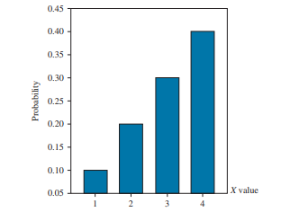
When selecting a shaded slip from Table P.1, the probability of selecting each possible outcome, $x=1,2,3$, and 4 is $0.25$. In the population of shaded slips the numeric values are equally likely. The probability of randomly selecting $X=2$ from the entire population, from the marginal $p d f$, is $P(X=2)=f_{X}(2)=0.2$. This is different from the conditional probability. Knowing that the slip is shaded tells us something about the probability of obtaining $X=2$. Such random variables are dependent in a statistical sense. Two random variables are statistically independent, or simply independent, if the conditional probability that $X=x$ given that $Y=y$ is the same as the unconditional probability that $X=x$. This means, if $X$ and $Y$ are independent random variables, then
$$
P(X=x \mid Y=y)=P(X=x)
$$
Equivalently, if $X$ and $Y$ are independent, then the conditional $p d f$ of $X$ given $Y=y$ is the same as the unconditional, or marginal, $p d f$ of $X$ alone.
$$
f(x \mid y)=\frac{f(x, y)}{f_{Y}(y)}=f_{X}(x)
$$
Solving (P.6) for the joint $p d f$, we can also say that $X$ and $Y$ are statistically independent if their joint $p d f$ factors into the product of their marginal $p d f \mathrm{~s}$
$$
P(X=x, Y=y)=f(x, y)=f_{X}(x) f_{Y}(y)=P(X=x) \times P(Y=y)
$$
If $(\mathbf{P} .5)$ or $(\mathbf{P} .7)$ is true for each and every pair of values $x$ and $y$, then $X$ and $Y$ are statistically independent. This result extends to more than two random variables. The rule allows us to check the independence of random variables $X$ and $Y$ in Table P.4. If (P.7) is violated for any pair of values, then $X$ and $Y$ are not statistically independent. Consider the pair of values $X=1$ and $Y=1$.
$$
P(X=1, Y=1)=f(1,1)=0.1 \neq f_{X}(1) f_{Y}(1)=P(X=1) \times P(Y=1)=0.1 \times 0.4=0.04
$$
The joint probability is $0.1$ and the product of the individual probabilities is $0.04$. Since these are not equal, we can conclude that $X$ and $Y$ are not statistically independent.
数学代写|计量经济学原理代写Principles of Econometrics代考|A Digression: Summation Notation
Throughout this book we will use a summation sign, denoted by the symbol $\sum$, to shorten algebraic expressions. Suppose the random variable $X$ takes the values $x_{1}, x_{2}, \ldots, x_{15}$. The sum of these values is $x_{1}+x_{2}+\cdots+x_{15}$. Rather than write this sum out each time we will represent it as $\sum_{i=1}^{15} x_{i}$, so that $\sum_{i=1}^{15} x_{i}=x_{1}+x_{2}+\cdots+x_{15}$. If we sum $n$ terms, a general number, then the summation will be $\sum_{i=1}^{n} x_{i}=x_{1}+x_{2}+\cdots+x_{n}$. In this notation
- The symbol $\sum$ is the capital Greek letter sigma and means “the sum of.”
- The letter $i$ is called the index of summation. This letter is arbitrary and may also appear as $t, j$, or $k$.
- The expression $\sum_{i=1}^{n} x_{i}$ is read “the sum of the terms $x_{i}$, from $i$ equals 1 to $n . “$
- The numbers 1 and $n$ are the lower limit and upper limit of summation.
The following rules apply to the summation operation.
Sum 1. The sum of $n$ values $x_{1}, \ldots, x_{n}$ is
$$
\sum_{i=1}^{n} x_{i}=x_{1}+x_{2}+\cdots+x_{n}
$$
Sum 2. If $a$ is a constant, then
$$
\sum_{i=1}^{n} a x_{i}=a \sum_{i=1}^{n} x_{i}
$$
Sum 3. If $a$ is a constant, then
$$
\sum_{i=1}^{n} a=a+a+\cdots+a=n a
$$
Sum 4. If $X$ and $Y$ are two variables, then
$$
\sum_{i=1}^{n}\left(x_{i}+y_{i}\right)=\sum_{i=1}^{n} x_{i}+\sum_{i=1}^{n} y_{i}
$$
Sum 5. If $X$ and $Y$ are two variables, then
$$
\sum_{i=1}^{n}\left(a x_{i}+b y_{i}\right)=a \sum_{i=1}^{n} x_{i}+b \sum_{i=1}^{n} y_{i}
$$
Sum 6. The arithmetic mean (average) of $n$ values of $X$ is
$$
\bar{x}=\frac{\sum_{i=1}^{n} x_{i}}{n}=\frac{x_{1}+x_{2}+\cdots+x_{n}}{n}
$$
Sum 7. A property of the arithmetic mean (average) is that
$$
\sum_{i=1}^{n}\left(x_{i}-\bar{x}\right)=\sum_{i=1}^{n} x_{i}-\sum_{i=1}^{n} \bar{x}=\sum_{i=1}^{n} x_{i}-n \bar{x}=\sum_{i=1}^{n} x_{i}-\sum_{i=1}^{n} x_{i}=0
$$
Sum 8. We often use an abbreviated form of the summation notation. For example, if $f(x)$ is a function of the values of $X$,
$$
\begin{aligned}
\sum_{i=1}^{n} f\left(x_{i}\right) &=f\left(x_{1}\right)+f\left(x_{2}\right)+\cdots+f\left(x_{n}\right) \
&=\sum_{i} f\left(x_{i}\right)(” \text { Sum over all values of the index } i \text { “) }\
&=\sum_{x} f(x)\left(” \text { Sum over all possible values of } X^{\prime \prime}\right)
\end{aligned}
$$
Sum 9. Several summation signs can be used in one expression. Suppose the variable $Y$ takes $n$ values and $X$ takes $m$ values, and let $f(x, y)=x+y$. Then the double summation of this function is
$$
\sum_{i=1}^{m} \sum_{j=1}^{n} f\left(x_{i}, y_{j}\right)=\sum_{i=1}^{m} \sum_{j=1}^{n}\left(x_{i}+y_{j}\right)
$$
To evaluate such expressions work from the innermost sum outward. First set $i=1$ and sum over all values of $j$, and so on. That is,
$$
\sum_{i=1}^{m} \sum_{j=1}^{n} f\left(x_{i}, y_{j}\right)=\sum_{i=1}^{m}\left[f\left(x_{i}, y_{1}\right)+f\left(x_{i}, y_{2}\right)+\cdots+f\left(x_{i}, y_{n}\right)\right]
$$
The order of summation does not matter, so
$$
\sum_{i=1}^{m} \sum_{j=1}^{n} f\left(x_{i}, y_{j}\right)=\sum_{j=1}^{n} \sum_{i=1}^{m} f\left(x_{i}, y_{j}\right)
$$
数学代写|计量经济学原理代写Principles of Econometrics代考|Calculating an Expected Value
For a discrete random variable the probability that $X$ takes the value $x$ is given by its $p d f f(x)$, $P(X=x)=f(x)$. The expected value in (P.8) can be written equivalently as
$$
\begin{aligned}
\mu_{X} &=E(X)=x_{1} f\left(x_{1}\right)+x_{2} f\left(x_{2}\right)+\cdots+x_{n} f\left(x_{n}\right) \
&=\sum_{i=1}^{n} x_{i} f\left(x_{i}\right)=\sum_{x} x f(x)
\end{aligned}
$$
Using (P.9), the expected value of $X$, the numeric value on a randomly drawn slip from Table P.1 is
$$
\mu_{x}=E(X)=\sum_{x=1}^{4} x f(x)=(1 \times 0.1)+(2 \times 0.2)+(3 \times 0.3)+(4 \times 0.4)=3
$$
What does this mean? Draw one “slip” at random from Table P.1, and observe its numerical value $X$. This constitutes an experiment. If we repeat this experiment many times, the values $x=1,2,3$, and 4 will appear $10 \%, 20 \%, 30 \%$, and $40 \%$ of the time, respectively. The arithmetic average of all the numerical values will approach $\mu_{X}=3$, as the number of experiments becomes large. The key point is that the expected value of the random variable is the average value that occurs in many repeated trials of an experiment.
For continuous random variables, the interpretation of the expected value of $X$ is unchanged it is the average value of $X$ if many values are obtained by repeatedly performing the underlying random experiment. ${ }^{4}$
计量经济学代考
数学代写|计量经济学原理代写Principles of Econometrics代考|Statistical Independence
当从表 P.1 中选择阴影滑动时,选择每个可能结果的概率,X=1,2,3, 4 是0.25. 在阴影滑动的总体中,数值的可能性相同。随机选择的概率X=2来自全体人口,来自边缘pdF, 是磷(X=2)=FX(2)=0.2. 这与条件概率不同。知道滑动是阴影告诉我们一些关于获得概率的信息X=2. 这种随机变量在统计意义上是依赖的。两个随机变量在统计上是独立的,或者只是独立的,如果条件概率X=X鉴于是=是与无条件概率相同X=X. 这意味着,如果X和是是独立的随机变量,那么
磷(X=X∣是=是)=磷(X=X)
等效地,如果X和是是独立的,那么有条件的pdF的X给定是=是与无条件的或边缘的相同,pdF的X独自的。
F(X∣是)=F(X,是)F是(是)=FX(X)
求解(P.6)关节pdF,我们也可以说X和是如果他们的联合是统计上独立的pdF因素到他们的边际产品pdF s
磷(X=X,是=是)=F(X,是)=FX(X)F是(是)=磷(X=X)×磷(是=是)
如果(磷.5)或者(磷.7)对每一对值都是正确的X和是, 然后X和是是统计独立的。这个结果扩展到两个以上的随机变量。该规则允许我们检查随机变量的独立性X和是在表 P.4 中。如果任何一对值都违反了 (P.7),那么X和是不是统计独立的。考虑这对值X=1和是=1.
磷(X=1,是=1)=F(1,1)=0.1≠FX(1)F是(1)=磷(X=1)×磷(是=1)=0.1×0.4=0.04
联合概率为0.1并且个体概率的乘积是0.04. 由于这些不相等,我们可以得出结论X和是不是统计独立的。
数学代写|计量经济学原理代写Principles of Econometrics代考|A Digression: Summation Notation
在本书中,我们将使用求和符号,用符号表示∑, 以缩短代数表达式。假设随机变量X取值X1,X2,…,X15. 这些值的总和是X1+X2+⋯+X15. 而不是每次都写出这个总和,我们将其表示为∑一世=115X一世, 以便∑一世=115X一世=X1+X2+⋯+X15. 如果我们总结n术语,一个通用数字,那么总和将是∑一世=1nX一世=X1+X2+⋯+Xn. 在这个符号中
- 符号∑是大写的希腊字母 sigma,意思是“总和”。
- 信一世称为求和指数。这封信是任意的,也可能显示为吨,j, 或者ķ.
- 表达方式∑一世=1nX一世读作“条款的总和X一世, 从一世等于 1 到n.“
- 数字 1 和n是求和的下限和上限。
以下规则适用于求和运算。
总和 1. 总和n价值观X1,…,Xn是
∑一世=1nX一世=X1+X2+⋯+Xn
总和 2. 如果一个是一个常数,那么
∑一世=1n一个X一世=一个∑一世=1nX一世
总和 3. 如果一个是一个常数,那么
∑一世=1n一个=一个+一个+⋯+一个=n一个
总和 4. 如果X和是是两个变量,那么
∑一世=1n(X一世+是一世)=∑一世=1nX一世+∑一世=1n是一世
总和 5. 如果X和是是两个变量,那么
∑一世=1n(一个X一世+b是一世)=一个∑一世=1nX一世+b∑一世=1n是一世
总和 6. 的算术平均值(平均值)n的值X是
X¯=∑一世=1nX一世n=X1+X2+⋯+Xnn
总和 7. 算术平均值(平均值)的一个性质是
∑一世=1n(X一世−X¯)=∑一世=1nX一世−∑一世=1nX¯=∑一世=1nX一世−nX¯=∑一世=1nX一世−∑一世=1nX一世=0
Sum 8. 我们经常使用求和符号的缩写形式。例如,如果F(X)是值的函数X,
∑一世=1nF(X一世)=F(X1)+F(X2)+⋯+F(Xn) =∑一世F(X一世)(” 对索引的所有值求和 一世 “) =∑XF(X)(” 对所有可能的值求和 X′′)
Sum 9. 在一个表达式中可以使用多个求和符号。假设变量是需要n价值观和X需要米值,并让F(X,是)=X+是. 那么这个函数的双重求和是
∑一世=1米∑j=1nF(X一世,是j)=∑一世=1米∑j=1n(X一世+是j)
评估这样的表达式从最里面的和向外工作。第一组一世=1并对所有值求和j, 等等。那是,
∑一世=1米∑j=1nF(X一世,是j)=∑一世=1米[F(X一世,是1)+F(X一世,是2)+⋯+F(X一世,是n)]
求和的顺序无关紧要,所以
∑一世=1米∑j=1nF(X一世,是j)=∑j=1n∑一世=1米F(X一世,是j)
数学代写|计量经济学原理代写Principles of Econometrics代考|Calculating an Expected Value
对于离散随机变量的概率X取值X由其给出pdFF(X), 磷(X=X)=F(X). (P.8) 中的期望值可以等效地写为
μX=和(X)=X1F(X1)+X2F(X2)+⋯+XnF(Xn) =∑一世=1nX一世F(X一世)=∑XXF(X)
使用(P.9),期望值X,从表 P.1 中随机抽取的单据上的数值为
μX=和(X)=∑X=14XF(X)=(1×0.1)+(2×0.2)+(3×0.3)+(4×0.4)=3
这是什么意思?从表 P.1 中随机抽取一张“纸条”,观察其数值X. 这构成了一个实验。如果我们多次重复这个实验,值X=1,2,3, 会出现 410%,20%,30%, 和40%的时间,分别。所有数值的算术平均值将接近μX=3,随着实验的数量变大。关键是随机变量的期望值是一个实验的多次重复试验中出现的平均值。
对于连续随机变量,期望值的解释X不变它是平均值X如果通过重复执行基础随机实验获得了许多值。4

统计代写请认准statistics-lab™. statistics-lab™为您的留学生涯保驾护航。
金融工程代写
金融工程是使用数学技术来解决金融问题。金融工程使用计算机科学、统计学、经济学和应用数学领域的工具和知识来解决当前的金融问题,以及设计新的和创新的金融产品。
非参数统计代写
非参数统计指的是一种统计方法,其中不假设数据来自于由少数参数决定的规定模型;这种模型的例子包括正态分布模型和线性回归模型。
广义线性模型代考
广义线性模型(GLM)归属统计学领域,是一种应用灵活的线性回归模型。该模型允许因变量的偏差分布有除了正态分布之外的其它分布。
术语 广义线性模型(GLM)通常是指给定连续和/或分类预测因素的连续响应变量的常规线性回归模型。它包括多元线性回归,以及方差分析和方差分析(仅含固定效应)。
有限元方法代写
有限元方法(FEM)是一种流行的方法,用于数值解决工程和数学建模中出现的微分方程。典型的问题领域包括结构分析、传热、流体流动、质量运输和电磁势等传统领域。
有限元是一种通用的数值方法,用于解决两个或三个空间变量的偏微分方程(即一些边界值问题)。为了解决一个问题,有限元将一个大系统细分为更小、更简单的部分,称为有限元。这是通过在空间维度上的特定空间离散化来实现的,它是通过构建对象的网格来实现的:用于求解的数值域,它有有限数量的点。边界值问题的有限元方法表述最终导致一个代数方程组。该方法在域上对未知函数进行逼近。[1] 然后将模拟这些有限元的简单方程组合成一个更大的方程系统,以模拟整个问题。然后,有限元通过变化微积分使相关的误差函数最小化来逼近一个解决方案。
tatistics-lab作为专业的留学生服务机构,多年来已为美国、英国、加拿大、澳洲等留学热门地的学生提供专业的学术服务,包括但不限于Essay代写,Assignment代写,Dissertation代写,Report代写,小组作业代写,Proposal代写,Paper代写,Presentation代写,计算机作业代写,论文修改和润色,网课代做,exam代考等等。写作范围涵盖高中,本科,研究生等海外留学全阶段,辐射金融,经济学,会计学,审计学,管理学等全球99%专业科目。写作团队既有专业英语母语作者,也有海外名校硕博留学生,每位写作老师都拥有过硬的语言能力,专业的学科背景和学术写作经验。我们承诺100%原创,100%专业,100%准时,100%满意。
随机分析代写
随机微积分是数学的一个分支,对随机过程进行操作。它允许为随机过程的积分定义一个关于随机过程的一致的积分理论。这个领域是由日本数学家伊藤清在第二次世界大战期间创建并开始的。
时间序列分析代写
随机过程,是依赖于参数的一组随机变量的全体,参数通常是时间。 随机变量是随机现象的数量表现,其时间序列是一组按照时间发生先后顺序进行排列的数据点序列。通常一组时间序列的时间间隔为一恒定值(如1秒,5分钟,12小时,7天,1年),因此时间序列可以作为离散时间数据进行分析处理。研究时间序列数据的意义在于现实中,往往需要研究某个事物其随时间发展变化的规律。这就需要通过研究该事物过去发展的历史记录,以得到其自身发展的规律。
回归分析代写
多元回归分析渐进(Multiple Regression Analysis Asymptotics)属于计量经济学领域,主要是一种数学上的统计分析方法,可以分析复杂情况下各影响因素的数学关系,在自然科学、社会和经济学等多个领域内应用广泛。
MATLAB代写
MATLAB 是一种用于技术计算的高性能语言。它将计算、可视化和编程集成在一个易于使用的环境中,其中问题和解决方案以熟悉的数学符号表示。典型用途包括:数学和计算算法开发建模、仿真和原型制作数据分析、探索和可视化科学和工程图形应用程序开发,包括图形用户界面构建MATLAB 是一个交互式系统,其基本数据元素是一个不需要维度的数组。这使您可以解决许多技术计算问题,尤其是那些具有矩阵和向量公式的问题,而只需用 C 或 Fortran 等标量非交互式语言编写程序所需的时间的一小部分。MATLAB 名称代表矩阵实验室。MATLAB 最初的编写目的是提供对由 LINPACK 和 EISPACK 项目开发的矩阵软件的轻松访问,这两个项目共同代表了矩阵计算软件的最新技术。MATLAB 经过多年的发展,得到了许多用户的投入。在大学环境中,它是数学、工程和科学入门和高级课程的标准教学工具。在工业领域,MATLAB 是高效研究、开发和分析的首选工具。MATLAB 具有一系列称为工具箱的特定于应用程序的解决方案。对于大多数 MATLAB 用户来说非常重要,工具箱允许您学习和应用专业技术。工具箱是 MATLAB 函数(M 文件)的综合集合,可扩展 MATLAB 环境以解决特定类别的问题。可用工具箱的领域包括信号处理、控制系统、神经网络、模糊逻辑、小波、仿真等。