数学代写|计量经济学原理代写Principles of Econometrics代考|Expected Values of Several Random Variables

statistics-lab™ 为您的留学生涯保驾护航在代写计量经济学Principles of Econometrics方面已经树立了自己的口碑, 保证靠谱, 高质且原创的统计Statistics代写服务。我们的专家在代写计量经济学Principles of Econometrics代写方面经验极为丰富，各种代写计量经济学Principles of Econometrics相关的作业也就用不着说。

我们提供的计量经济学Principles of Econometrics及其相关学科的代写，服务范围广, 其中包括但不限于:

Statistical Inference 统计推断
Statistical Computing 统计计算
Advanced Probability Theory 高等概率论
Advanced Mathematical Statistics 高等数理统计学
(Generalized) Linear Models 广义线性模型
Statistical Machine Learning 统计机器学习
Longitudinal Data Analysis 纵向数据分析
Foundations of Data Science 数据科学基础

数学代写|计量经济学原理代写Principles of Econometrics代考|Expected Values of Several Random Variables

数学代写|计量经济学原理代写Principles of Econometrics代考|Covariance Between Two Random Variables

The covariance between $X$ and $Y$ is a measure of linear association between them. Think about two continuous variables, such as height and weight of children. We expect that there is an association between height and weight, with taller than average children tending to weigh more than the average. The product of $X$ minus its mean times $Y$ minus its mean is
$$
\left(X-\mu_{X}\right)\left(Y-\mu_{Y}\right)
$$
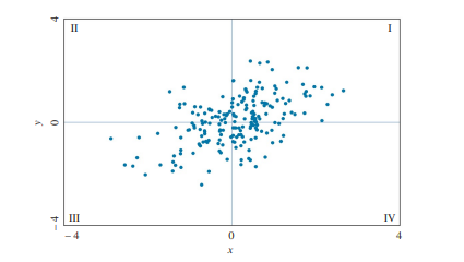
In Figure P.4, we plot values ( $x$ and $y$ ) of $X$ and $Y$ that have been constructed so that $E(X)=E(Y)=0$.

The $x$ and $y$ values of $X$ and $Y$ fall predominately in quadrants I and III, so that the arithmetic average of the values $\left(x-\mu_{X}\right)\left(y-\mu_{Y}\right)$ is positive. We define the covariance between two random variables as the expected (population average) value of the product in (P.17).
$$
\operatorname{cov}(X, Y)=\sigma_{X Y}=E\left[\left(X-\mu_{X}\right)\left(Y-\mu_{Y}\right)\right]=E(X Y)-\mu_{X} \mu_{Y}
$$
We use the letters “cov” to represent covariance, and $\operatorname{cov}(X, Y)$ is read as “the covariance between $X$ and $Y$,” where $X$ and $Y$ are random variables. The covariance $\sigma_{X Y}$ of the random variables underlying Figure P.4 is positive, which tells us that when the values $x$ are greater

than $\mu_{X}$, then the values $y$ also tend to be greater than $\mu_{Y}$; and when the values $x$ are below $\mu_{X}$, then the values $y$ also tend to be less than $\mu_{Y}$. If the random variables values tend primarily to fall in quadrants II and IV, then $\left(x-\mu_{X}\right)\left(y-\mu_{Y}\right)$ will tend to be negative and $\sigma_{X Y}$ will be negative. If the random variables values are spread evenly across the four quadrants, and show neither positive nor negative association, then the covariance is zero. The sign of $\sigma_{X Y}$ tells us whether the two random variables $X$ and $Y$ are positively associated or negatively associated.

Interpreting the actual value of $\sigma_{X Y}$ is difficult because $X$ and $Y$ may have different units of measurement. Scaling the covariance by the standard deviations of the variables eliminates the units of measurement, and defines the correlation between $X$ and $Y$
$$
\rho=\frac{\operatorname{cov}(X, Y)}{\sqrt{\operatorname{var}(X)} \sqrt{\operatorname{var}(Y)}}=\frac{\sigma_{X Y}}{\sigma_{X} \sigma_{Y}}
$$
As with the covariance, the correlation $\rho$ between two random variables measures the degree of linear association between them. However, unlike the covariance, the correlation must lie between $-1$ and 1. Thus, the correlation between $X$ and $Y$ is 1 or $-1$ if $X$ is a perfect positive or negative linear function of $Y$. If there is no linear association between $X$ and $Y$, then $\operatorname{cov}(X, Y)=0$ and $\rho=0$. For other values of correlation the magnitude of the absolute value $|\rho|$ indicates the “strength” of the linear association between the values of the random variables. In Figure P.4, the correlation between $X$ and $Y$ is $\rho=0.5$.

数学代写|计量经济学原理代写Principles of Econometrics代考|Conditional Variance

The unconditional variance of a discrete random variable $X$ is
$$
\operatorname{var}(X)=\sigma_{X}^{2}=E\left[\left(X-\mu_{X}\right)^{2}\right]=\sum_{x}\left(x-\mu_{X}\right)^{2} f(x)
$$
It measures how much variation there is in $X$ around the unconditional mean of $X_{\text {, }} \mu_{X}$. For example, the unconditional variance $\operatorname{var}(W A G E)$ measures the variation in $W A G E$ around the unconditional mean $E(W A G E)$. In (P.13) we show that equivalently
$$
\operatorname{var}(X)=\sigma_{X}^{2}=E\left(X^{2}\right)-\mu_{X}^{2}=\sum_{x} x^{2} f(x)-\mu_{X}^{2}
$$
In Section P.6.1 we discussed how to answer the question “What is the mean wage of a person who has 16 years of education?” Now we ask “How much variation is there in wages for a person who has 16 years of education?* The answer to this question is given by the conditional variance, $\operatorname{var}(W A G E \mid E D U C=16)$. The conditional variance measures the variation in WAGE around the conditional mean $E(W A G E \mid E D U C=16)$ for individuals with 16 years of education. The conditional variance of WAGE for individuals with 16 years of education is the average squared difference in the population between WAGE and the conditional mean of WAGE,
$$
\underbrace{\operatorname{var}(W A G E \mid E D U C=16)}{\text {conditional variance }}=E\left{[\underbrace{E D A G E-\underbrace{E(W A G E \mid E D U C=16)}}{\text {conditional mean }}]^{2} \mid E D U=16\right}
$$
To obtain the conditional variance we modify the definitions of variance in equations (P.26) and (P.27); replace the unconditional mean $E(X)=\mu_{X}$ with the conditional mean $E(X \mid Y=y)$, and the unconditional $p d f f(x)$ with the conditional $p d f f(x \mid y)$. Then
$$
\operatorname{var}(X \mid Y=y)=E\left{[X-E(X \mid Y=y)]^{2} \mid Y=y\right}=\sum_{x}(x-E(X \mid Y=y))^{2} f(x \mid y)
$$
or
$$
\operatorname{var}(X \mid Y=y)=E\left(X^{2} \mid Y=y\right)-[E(X \mid Y=y)]^{2}=\sum_{x} x^{2} f(x \mid y)-[E(X \mid Y=y)]^{2}
$$

数学代写|计量经济学原理代写Principles of Econometrics代考|Proof of the Law of Iterated Expectations

Proof of the Law of Iterated Expectations To prove the Law of Iterated Expectations we make use of relationships between joint, marginal, and conditional $p d f$ s that we introduced in Section P.3. In Section P.3.1 we discussed marginal distributions. Given a joint $p d f$ $f(x, y)$ we can obtain the marginal pdf of $y$ alone $f_{Y}(y)$ by summing, for each $y$, the joint $p d f$ $f(x, y)$ across all values of the variable we wish to eliminate, in this case $x$. That is, for $Y$ and $X$,
$$
\begin{aligned}
&f(y)=f_{Y}(y)=\sum_{x} f(x, y) \
&f(x)=f_{X}(x)=\sum_{y} f(x, y)
\end{aligned}
$$
Because $f()$ is used to represent $p d f$ s in general, sometimes we will put a subscript, $X$ or $Y$, to be very clear about which variable is random.
Using equation (P.4) we can define the conditional pdf of $y$ given $X=x$ as
$$
f(y \mid x)=\frac{f(x, y)}{f_{X}(x)}
$$
Rearrange this expression to obtain
$$
f(x, y)=f(y \mid x) f_{X}(x)
$$
A joint $p d f$ is the product of the conditional $p d f$ and the $p d f$ of the conditioning variable.

To show that the Law of Iterated Expectations is true ${ }^{8}$ we begin with the definition of the expected value of $Y$, and operate with the summation.
$$
\begin{aligned}
E(Y) &=\sum_{y} y f(y)=\sum_{y} y\left[\sum_{x} f(x, y)\right] & & {[\text { substitute for } f(y)] } \
&=\sum_{y} y\left[\sum_{x} f(y \mid x) f_{X}(x)\right] & & {[\text { substitute for } f(x, y)] } \
&=\sum_{x}\left[\sum_{y} y f(y \mid x)\right] f_{X}(x) & & \text { [change order of summation] } \
&=\sum_{x} E(Y \mid x) f_{X}(x) & & {[\text { recognize the conditional expectation] }} \
&=E_{X}[E(Y \mid X)] & &
\end{aligned}
$$
While this result may seem an esoteric oddity it is very important and widely used in modern econometrics.

计量经济学代考

数学代写|计量经济学原理代写Principles of Econometrics代考|Covariance Between Two Random Variables

之间的协方差X和是是它们之间线性关联的度量。考虑两个连续变量，例如儿童的身高和体重。我们预计身高和体重之间存在关联，高于平均水平的儿童往往体重高于平均水平。的产品X减去平均时间是减去它的平均值是

(X−μX)(是−μ是)
在图 P.4 中，我们绘制了值 (X和是）的X和是已被构造成和(X)=和(是)=0.

这X和是的值X和是主要落在第一象限和第三象限，因此这些值的算术平均值(X−μX)(是−μ是)是积极的。我们将两个随机变量之间的协方差定义为（P.17）中产品的预期（总体平均值）值。

这⁡(X,是)=σX是=和[(X−μX)(是−μ是)]=和(X是)−μXμ是
我们使用字母“cov”来表示协方差，并且这⁡(X,是)被读作“之间的协方差X和是，“ 在哪里X和是是随机变量。协方差σX是图 P.4 下的随机变量的为正数，这告诉我们，当值X更大

比μX, 那么值是也往往大于μ是; 当值X在下面μX, 那么值是也往往小于μ是. 如果随机变量值主要落在象限 II 和 IV 中，那么(X−μX)(是−μ是)将趋于消极和σX是将是负面的。如果随机变量值均匀地分布在四个象限中，并且既不显示正相关也不显示负相关，则协方差为零。的标志σX是告诉我们两个随机变量是否X和是是正相关还是负相关。

解释实际值σX是很难，因为X和是可能有不同的计量单位。通过变量的标准偏差缩放协方差消除了测量单位，并定义了之间的相关性X和是

ρ=这⁡(X,是)曾是⁡(X)曾是⁡(是)=σX是σXσ是
与协方差一样，相关性ρ在两个随机变量之间测量它们之间的线性关联程度。然而，与协方差不同的是，相关性必须介于−1和 1. 因此，之间的相关性X和是是 1 或−1如果X是一个完美的正或负线性函数是. 如果两者之间没有线性关联X和是，然后这⁡(X,是)=0和ρ=0. 对于其他相关值，绝对值的大小|ρ|表示随机变量值之间线性关联的“强度”。在图 P.4 中，X和是是ρ=0.5.

数学代写|计量经济学原理代写Principles of Econometrics代考|Conditional Variance

离散随机变量的无条件方差X是

曾是⁡(X)=σX2=和[(X−μX)2]=∑X(X−μX)2F(X)
它测量有多少变化X围绕无条件均值X, μX. 例如，无条件方差曾是⁡(在一个G和)测量变化在一个G和围绕无条件均值和(在一个G和). 在（P.13）中，我们等价地证明了

曾是⁡(X)=σX2=和(X2)−μX2=∑XX2F(X)−μX2
在第 P.6.1 节中，我们讨论了如何回答“一个受过 16 年教育的人的平均工资是多少？”这个问题。现在我们问“受过 16 年教育的人的工资有多少变化？* 这个问题的答案由条件方差给出，曾是⁡(在一个G和∣和D在C=16). 条件方差衡量 WAGE 围绕条件均值的变化和(在一个G和∣和D在C=16)适用于受过 16 年教育的个人。受教育年限为 16 年的个人的 WAGE 条件方差是 WAGE 与 WAGE 条件均值之间人口的平均平方差，

\underbrace{\operatorname{var}(W A G E \mid E D U C=16)}{\text {条件方差}}=E\left{[\underbrace{E D A G E-\underbrace{E(W A G E \mid E D U C=16)} }{\text {条件均值}}]^{2} \mid E D U=16\right}\underbrace{\operatorname{var}(W A G E \mid E D U C=16)}{\text {条件方差}}=E\left{[\underbrace{E D A G E-\underbrace{E(W A G E \mid E D U C=16)} }{\text {条件均值}}]^{2} \mid E D U=16\right}
为了获得条件方差，我们修改了方程 (P.26) 和 (P.27) 中的方差定义；替换无条件均值和(X)=μX条件均值和(X∣是=是), 和无条件的pdFF(X)有条件的pdFF(X∣是). 然后

\operatorname{var}(X \mid Y=y)=E\left{[XE(X \mid Y=y)]^{2} \mid Y=y\right}=\sum_{x}(xE( X \mid Y=y))^{2} f(x \mid y)\operatorname{var}(X \mid Y=y)=E\left{[XE(X \mid Y=y)]^{2} \mid Y=y\right}=\sum_{x}(xE( X \mid Y=y))^{2} f(x \mid y)
或者

曾是⁡(X∣是=是)=和(X2∣是=是)−[和(X∣是=是)]2=∑XX2F(X∣是)−[和(X∣是=是)]2

数学代写|计量经济学原理代写Principles of Econometrics代考|Proof of the Law of Iterated Expectations

迭代期望定律的证明为了证明迭代期望定律，我们利用联合、边际和条件之间的关系pdF我们在第 P.3 节中介绍的 s。在第 P.3.1 节中，我们讨论了边际分布。给定一个联合pdF F(X,是)我们可以得到边际pdf是独自的F是(是)通过求和，对于每个是，关节pdF F(X,是)在我们希望消除的变量的所有值中，在这种情况下X. 也就是说，对于是和X,

F(是)=F是(是)=∑XF(X,是) F(X)=FX(X)=∑是F(X,是)
因为F()用来表示pdFs 一般情况下，有时我们会放一个下标，X或者是，非常清楚哪个变量是随机的。
使用等式（P.4），我们可以定义条件 pdf是给定X=X作为

F(是∣X)=F(X,是)FX(X)
重新排列这个表达式以获得

F(X,是)=F(是∣X)FX(X)
结合点pdF是条件的乘积pdF和pdF的条件变量。

证明迭代期望定律是正确的8我们从期望值的定义开始是, 并进行求和运算。

和(是)=∑是是F(是)=∑是是[∑XF(X,是)][ 替代品 F(是)] =∑是是[∑XF(是∣X)FX(X)][ 替代品 F(X,是)] =∑X[∑是是F(是∣X)]FX(X) [改变求和顺序] =∑X和(是∣X)FX(X)[ 认识条件期望] =和X[和(是∣X)]
虽然这个结果可能看起来很奇怪，但它在现代计量经济学中非常重要并被广泛使用。

数学代写|计量经济学原理代写Principles of Econometrics代考请认准statistics-lab™

统计代写请认准statistics-lab™. statistics-lab™为您的留学生涯保驾护航。

金融工程代写

金融工程是使用数学技术来解决金融问题。金融工程使用计算机科学、统计学、经济学和应用数学领域的工具和知识来解决当前的金融问题，以及设计新的和创新的金融产品。

非参数统计代写

非参数统计指的是一种统计方法，其中不假设数据来自于由少数参数决定的规定模型；这种模型的例子包括正态分布模型和线性回归模型。

广义线性模型代考

广义线性模型（GLM）归属统计学领域，是一种应用灵活的线性回归模型。该模型允许因变量的偏差分布有除了正态分布之外的其它分布。

术语广义线性模型（GLM）通常是指给定连续和/或分类预测因素的连续响应变量的常规线性回归模型。它包括多元线性回归，以及方差分析和方差分析（仅含固定效应）。

有限元方法代写

有限元方法（FEM）是一种流行的方法，用于数值解决工程和数学建模中出现的微分方程。典型的问题领域包括结构分析、传热、流体流动、质量运输和电磁势等传统领域。

有限元是一种通用的数值方法，用于解决两个或三个空间变量的偏微分方程（即一些边界值问题）。为了解决一个问题，有限元将一个大系统细分为更小、更简单的部分，称为有限元。这是通过在空间维度上的特定空间离散化来实现的，它是通过构建对象的网格来实现的：用于求解的数值域，它有有限数量的点。边界值问题的有限元方法表述最终导致一个代数方程组。该方法在域上对未知函数进行逼近。[1] 然后将模拟这些有限元的简单方程组合成一个更大的方程系统，以模拟整个问题。然后，有限元通过变化微积分使相关的误差函数最小化来逼近一个解决方案。

tatistics-lab作为专业的留学生服务机构，多年来已为美国、英国、加拿大、澳洲等留学热门地的学生提供专业的学术服务，包括但不限于Essay代写，Assignment代写，Dissertation代写，Report代写，小组作业代写，Proposal代写，Paper代写，Presentation代写，计算机作业代写，论文修改和润色，网课代做，exam代考等等。写作范围涵盖高中，本科，研究生等海外留学全阶段，辐射金融，经济学，会计学，审计学，管理学等全球99%专业科目。写作团队既有专业英语母语作者，也有海外名校硕博留学生，每位写作老师都拥有过硬的语言能力，专业的学科背景和学术写作经验。我们承诺100%原创，100%专业，100%准时，100%满意。

随机分析代写

随机微积分是数学的一个分支，对随机过程进行操作。它允许为随机过程的积分定义一个关于随机过程的一致的积分理论。这个领域是由日本数学家伊藤清在第二次世界大战期间创建并开始的。

时间序列分析代写

随机过程，是依赖于参数的一组随机变量的全体，参数通常是时间。随机变量是随机现象的数量表现，其时间序列是一组按照时间发生先后顺序进行排列的数据点序列。通常一组时间序列的时间间隔为一恒定值（如1秒，5分钟，12小时，7天，1年），因此时间序列可以作为离散时间数据进行分析处理。研究时间序列数据的意义在于现实中，往往需要研究某个事物其随时间发展变化的规律。这就需要通过研究该事物过去发展的历史记录，以得到其自身发展的规律。

回归分析代写

多元回归分析渐进（Multiple Regression Analysis Asymptotics）属于计量经济学领域，主要是一种数学上的统计分析方法，可以分析复杂情况下各影响因素的数学关系，在自然科学、社会和经济学等多个领域内应用广泛。

MATLAB代写

MATLAB 是一种用于技术计算的高性能语言。它将计算、可视化和编程集成在一个易于使用的环境中，其中问题和解决方案以熟悉的数学符号表示。典型用途包括：数学和计算算法开发建模、仿真和原型制作数据分析、探索和可视化科学和工程图形应用程序开发，包括图形用户界面构建MATLAB 是一个交互式系统，其基本数据元素是一个不需要维度的数组。这使您可以解决许多技术计算问题，尤其是那些具有矩阵和向量公式的问题，而只需用 C 或 Fortran 等标量非交互式语言编写程序所需的时间的一小部分。MATLAB 名称代表矩阵实验室。MATLAB 最初的编写目的是提供对由 LINPACK 和 EISPACK 项目开发的矩阵软件的轻松访问，这两个项目共同代表了矩阵计算软件的最新技术。MATLAB 经过多年的发展，得到了许多用户的投入。在大学环境中，它是数学、工程和科学入门和高级课程的标准教学工具。在工业领域，MATLAB 是高效研究、开发和分析的首选工具。MATLAB 具有一系列称为工具箱的特定于应用程序的解决方案。对于大多数 MATLAB 用户来说非常重要，工具箱允许您学习和应用专业技术。工具箱是 MATLAB 函数（M 文件）的综合集合，可扩展 MATLAB 环境以解决特定类别的问题。可用工具箱的领域包括信号处理、控制系统、神经网络、模糊逻辑、小波、仿真等。

R语言代写	问卷设计与分析代写
PYTHON代写	回归分析与线性模型代写
MATLAB代写	方差分析与试验设计代写
STATA代写	机器学习/统计学习代写
SPSS代写	计量经济学代写
EVIEWS代写	时间序列分析代写
EXCEL代写	深度学习代写
SQL代写	各种数据建模与可视化代写