如果你也在 怎样代写黎曼几何Riemannian geometry这个学科遇到相关的难题,请随时右上角联系我们的24/7代写客服。
黎曼几何是研究黎曼流形的微分几何学分支,黎曼流形是具有黎曼公制的光滑流形,即在每一点的切线空间上有一个内积,从一点到另一点平滑变化。
statistics-lab™ 为您的留学生涯保驾护航 在代写黎曼几何Riemannian geometry方面已经树立了自己的口碑, 保证靠谱, 高质且原创的统计Statistics代写服务。我们的专家在代写黎曼几何Riemannian geometry代写方面经验极为丰富,各种代写黎曼几何Riemannian geometry相关的作业也就用不着说。
我们提供的黎曼几何Riemannian geometry及其相关学科的代写,服务范围广, 其中包括但不限于:
- Statistical Inference 统计推断
- Statistical Computing 统计计算
- Advanced Probability Theory 高等概率论
- Advanced Mathematical Statistics 高等数理统计学
- (Generalized) Linear Models 广义线性模型
- Statistical Machine Learning 统计机器学习
- Longitudinal Data Analysis 纵向数据分析
- Foundations of Data Science 数据科学基础
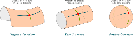
数学代写|黎曼几何代写Riemannian geometry代考|Negative Curvature: The Hyperbolic Plane
The negative constant curvature model is the hyperbolic plane $H_{r}^{2}$ obtained as the surface of $\mathbb{R}^{3}$, endowed with the hyperbolic metric, defined as the zero level set of the function
$$
a(x, y, z)=x^{2}+y^{2}-z^{2}+r^{2} .
$$
Indeed, this surface is a two-fold hyperboloid, so we can restrict our attention to the set of points $H_{r}^{2}=a^{-1}(0) \cap{z>0}$.
In analogy with the positive constant curvature model (which is the set of points in $\mathbb{R}^{3}$ whose Euclidean norm is constant) the negative constant curvature model can be seen as the set of points whose hyperbolic norm is constant in $\mathbb{R}^{3}$. In other words,
$$
H_{r}^{2}=\left{q=(x, y, z) \in \mathbb{R}^{3} \mid|q|_{h}^{2}=-r^{2}\right} \cap{z>0}
$$
The hyperbolic Gauss map associated with this surface can be easily computed, since it is explicitly given by
$$
\mathcal{N}: H_{r}^{2} \rightarrow H^{2}, \quad \mathcal{N}(q)=\frac{1}{r} \nabla_{q} a
$$
Exercise 1.63 Prove that the Gaussian curvature of $H_{r}^{2}$ is $\kappa=-1 / r^{2}$ at every point $q \in H_{r}^{2}$.
We can now discuss the structure of geodesics and curves with constant geodesic curvature on the hyperbolic space. We start with a result that can be proved in an analogous way to Proposition $1.60$. The proof is left to the reader.
Proposition 1.64 Let $\gamma:[0, T] \rightarrow H_{r}^{2}$ be a curve with unit speed and constant geodesic curvature equal to $c \in \mathbb{R}$. For every vector $w \in \mathbb{R}^{3}$, the function $\alpha(t)=\langle\dot{\gamma}(t) \mid w\rangle_{h}$ is a solution of the differential equation
$$
\ddot{\alpha}(t)+\left(c^{2}-\frac{1}{r^{2}}\right) \alpha(t)=0 .
$$
数学代写|黎曼几何代写Riemannian geometry代考|Tangent Vectors and Vector Fields
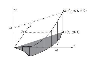
Let $M$ be a smooth $n$-dimensional manifold and let $\gamma_{1}, \gamma_{2}: I \rightarrow M$ be two smooth curves based at $q=\gamma_{1}(0)=\gamma_{2}(0) \in M$. We say that $\gamma_{1}$ and $\gamma_{2}$ are equivalent if they have the same first-order Taylor polynomial in some (or, equivalently, in every) coordinate chart. This defines an equivalence relation on the space of smooth curves based at $q$.
Definition 2.1 Let $M$ be a smooth $n$-dimensional manifold and let $\gamma: I \rightarrow$ $M$ be a smooth curve such that $\gamma(0)=q \in M$. Its tangent vector at $q=\gamma(0)$, denoted by
$$
\left.\frac{d}{d t}\right|_{t=0} \gamma(t) \quad \text { or } \quad \dot{\gamma}(0),
$$
is the equivalence class in the space of all smooth curves in $M$ such that $\gamma(0)=$ $q$ (with respect to the equivalence relation defined above).
It is easy to check, using the chain rule, that this definition is well posed (i.e., it does not depend on the representative curve).
Definition $2.2$ Let $M$ be a smooth $n$-dimensional manifold. The tangent space to $M$ at a point $q \in M$ is the set
$$
T_{q} M:=\left{\left.\frac{d}{d t}\right|{t=0} \gamma(t) \mid \gamma: I \rightarrow M \text { smooth, } \gamma(0)=q\right} . $$ It is a standard fact that $T{q} M$ has a natural structure of an $n$-dimensional vector space, where $n=\operatorname{dim} M$.
Definition 2.3 A smooth vector field on a smooth manifold $M$ is a smooth map
$$
X: q \mapsto X(q) \in T_{q} M
$$
that associates with every point $q$ in $M$ a tangent vector at $q$. We denote by $\operatorname{Vec}(M)$ the set of smooth vector fields on $M$.
In coordinates we can write $X=\sum_{i=1}^{n} X^{i}(x) \partial / \partial x_{i}$, and the vector field is smooth if its components $X^{i}(x)$ are smooth functions. The value of a vector field $X$ at a point $q$ is denoted, in what follows, by both $X(q)$ and $\left.X\right|_{q}$.
数学代写|黎曼几何代写Riemannian geometry代考|Flow of a Vector Field
Given a complete vector field $X \in \operatorname{Vec}(M)$ we can consider the family of maps
$$
\phi_{t}: M \rightarrow M, \quad \phi_{t}(q)=\gamma(t ; q), \quad t \in \mathbb{R}{2} $$ where $\gamma(t ; q)$ is the integral curve of $X$ starting at $q$ when $t=0$. By Theorem $2.5$ it follows that the map $$ \phi: \mathbb{R} \times M \rightarrow M{,} \quad \phi(t, q)=\phi_{t}(q)
$$
is smooth in both variables and the family $\left{\phi_{t}, t \in \mathbb{R}\right}$ is a one-parametric subgroup of Diff $(M)$; namely, it satisfies the following identities:
$$
\begin{aligned}
\phi_{0} &=\mathrm{Id}{+} \ \phi{t} \circ \phi_{s} &=\phi_{s} \circ \phi_{t}=\phi_{t+s}, \quad \forall t, s \subset \mathbb{R}, \
\left(\phi_{t}\right)^{-1} &=\phi_{-t}, \quad \forall t \in \mathbb{R} .
\end{aligned}
$$
Moreover, by construction, we have
$$
\frac{\partial \phi_{t}(q)}{\partial t}=X\left(\phi_{t}(q)\right), \quad \phi_{0}(q)=q, \quad \forall q \in M
$$
The family of maps $\phi_{t}$ defined by $(2.5)$ is called the flow generated by $X$. For the flow $\phi_{t}$ of a vector field $X$ it is convenient to use the exponential notation $\phi_{t}:=e^{t X}$, for every $t \in \mathbb{R}$. Using this notation, the group properties (2.6) take the form
$$
\begin{gathered}
e^{0 X}=\mathrm{Id}, \quad e^{t X} \circ e^{s X}=e^{s X} \circ e^{t X}=e^{(t+s) X}, \quad\left(e^{t X}\right)^{-1}=e^{-t X} \
\frac{d}{d t} e^{t X}(q)=X\left(e^{t X}(q)\right), \quad \forall q \in M
\end{gathered}
$$
Remark $2.8$ When $X(x)=A x$ is a linear vector field on $\mathbb{R}^{n}$, where $A$ is an $n \times n$ matrix, the corresponding flow $\phi_{t}$ is the matrix exponential $\phi_{t}(x)=e^{t A} x$.
黎曼几何代考
数学代写|黎曼几何代写Riemannian geometry代考|Negative Curvature: The Hyperbolic Plane
负常曲率模型是双曲平面Hr2作为表面获得R3, 赋予双曲线度量,定义为函数的零水平集
一个(X,是,和)=X2+是2−和2+r2.
事实上,这个曲面是一个二重双曲面,所以我们可以将注意力限制在点集上Hr2=一个−1(0)∩和>0.
类似于正常曲率模型(即R3其欧几里得范数是常数)负常数曲率模型可以看作是双曲范数在R3. 换句话说,
H_{r}^{2}=\left{q=(x, y, z) \in \mathbb{R}^{3} \mid|q|_{h}^{2}=-r^{ 2}\right} \cap{z>0}H_{r}^{2}=\left{q=(x, y, z) \in \mathbb{R}^{3} \mid|q|_{h}^{2}=-r^{ 2}\right} \cap{z>0}
与该表面相关的双曲高斯图可以很容易地计算出来,因为它明确地由下式给出
ñ:Hr2→H2,ñ(q)=1r∇q一个
练习 1.63 证明高斯曲率Hr2是ķ=−1/r2在每一点q∈Hr2.
我们现在可以讨论在双曲空间上具有恒定测地曲率的测地线和曲线的结构。我们从一个可以以类似于命题的方式证明的结果开始1.60. 证明留给读者。
命题 1.64 让C:[0,吨]→Hr2是一条单位速度和恒定测地曲率等于的曲线C∈R. 对于每个向量在∈R3, 功能一个(吨)=⟨C˙(吨)∣在⟩H是微分方程的解
一个¨(吨)+(C2−1r2)一个(吨)=0.
数学代写|黎曼几何代写Riemannian geometry代考|Tangent Vectors and Vector Fields
让米做一个光滑的n维流形并让C1,C2:我→米是两条基于的平滑曲线q=C1(0)=C2(0)∈米. 我们说C1和C2如果它们在某些(或等效地,在每个)坐标图中具有相同的一阶泰勒多项式,则它们是等价的。这定义了基于平滑曲线空间的等价关系q.
定义 2.1 让米做一个光滑的n维流形并让C:我→ 米是一条平滑曲线,使得C(0)=q∈米. 它的切向量在q=C(0),表示为
dd吨|吨=0C(吨) 或者 C˙(0),
是所有平滑曲线空间中的等价类米这样C(0)= q(关于上面定义的等价关系)。
使用链式法则很容易检查这个定义是否恰当(即,它不依赖于代表曲线)。
定义2.2让米做一个光滑的n维流形。的切线空间米在某一点q∈米是集合
T_{q} M:=\left{\left.\frac{d}{d t}\right|{t=0} \gamma(t) \mid \gamma: I \rightarrow M \text { smooth, } \伽马(0)=q\right} 。T_{q} M:=\left{\left.\frac{d}{d t}\right|{t=0} \gamma(t) \mid \gamma: I \rightarrow M \text { smooth, } \伽马(0)=q\right} 。一个标准的事实是吨q米有一个自然的结构n维向量空间,其中n=暗淡米.
定义 2.3 光滑流形上的光滑矢量场米是一张光滑的地图
X:q↦X(q)∈吨q米
与每一点相关联q在米一个切向量在q. 我们表示一个东西(米)上的平滑向量场集米.
在坐标中我们可以写X=∑一世=1nX一世(X)∂/∂X一世,并且向量场是平滑的,如果它的分量X一世(X)是平滑函数。向量场的值X在某一点q在下文中,由两者表示X(q)和X|q.
数学代写|黎曼几何代写Riemannian geometry代考|Flow of a Vector Field
给定一个完整的向量场X∈一个东西(米)我们可以考虑地图族
φ吨:米→米,φ吨(q)=C(吨;q),吨∈R2在哪里C(吨;q)是积分曲线X开始于q什么时候吨=0. 按定理2.5随之而来的是地图
φ:R×米→米,φ(吨,q)=φ吨(q)
在变量和家庭中都是平滑的\left{\phi_{t}, t \in \mathbb{R}\right}\left{\phi_{t}, t \in \mathbb{R}\right}是 Diff 的单参数子群(米); 即,它满足以下恒等式:
φ0=我d+ φ吨∘φs=φs∘φ吨=φ吨+s,∀吨,s⊂R, (φ吨)−1=φ−吨,∀吨∈R.
此外,通过构建,我们有
∂φ吨(q)∂吨=X(φ吨(q)),φ0(q)=q,∀q∈米
地图家族φ吨被定义为(2.5)被称为产生的流X. 对于流量φ吨向量场的X使用指数符号很方便φ吨:=和吨X, 对于每个吨∈R. 使用这种表示法,群属性 (2.6) 采用以下形式
和0X=我d,和吨X∘和sX=和sX∘和吨X=和(吨+s)X,(和吨X)−1=和−吨X dd吨和吨X(q)=X(和吨X(q)),∀q∈米
评论2.8什么时候X(X)=一个X是一个线性向量场Rn, 在哪里一个是一个n×n矩阵,对应流φ吨是矩阵指数φ吨(X)=和吨一个X.

统计代写请认准statistics-lab™. statistics-lab™为您的留学生涯保驾护航。
金融工程代写
金融工程是使用数学技术来解决金融问题。金融工程使用计算机科学、统计学、经济学和应用数学领域的工具和知识来解决当前的金融问题,以及设计新的和创新的金融产品。
非参数统计代写
非参数统计指的是一种统计方法,其中不假设数据来自于由少数参数决定的规定模型;这种模型的例子包括正态分布模型和线性回归模型。
广义线性模型代考
广义线性模型(GLM)归属统计学领域,是一种应用灵活的线性回归模型。该模型允许因变量的偏差分布有除了正态分布之外的其它分布。
术语 广义线性模型(GLM)通常是指给定连续和/或分类预测因素的连续响应变量的常规线性回归模型。它包括多元线性回归,以及方差分析和方差分析(仅含固定效应)。
有限元方法代写
有限元方法(FEM)是一种流行的方法,用于数值解决工程和数学建模中出现的微分方程。典型的问题领域包括结构分析、传热、流体流动、质量运输和电磁势等传统领域。
有限元是一种通用的数值方法,用于解决两个或三个空间变量的偏微分方程(即一些边界值问题)。为了解决一个问题,有限元将一个大系统细分为更小、更简单的部分,称为有限元。这是通过在空间维度上的特定空间离散化来实现的,它是通过构建对象的网格来实现的:用于求解的数值域,它有有限数量的点。边界值问题的有限元方法表述最终导致一个代数方程组。该方法在域上对未知函数进行逼近。[1] 然后将模拟这些有限元的简单方程组合成一个更大的方程系统,以模拟整个问题。然后,有限元通过变化微积分使相关的误差函数最小化来逼近一个解决方案。
tatistics-lab作为专业的留学生服务机构,多年来已为美国、英国、加拿大、澳洲等留学热门地的学生提供专业的学术服务,包括但不限于Essay代写,Assignment代写,Dissertation代写,Report代写,小组作业代写,Proposal代写,Paper代写,Presentation代写,计算机作业代写,论文修改和润色,网课代做,exam代考等等。写作范围涵盖高中,本科,研究生等海外留学全阶段,辐射金融,经济学,会计学,审计学,管理学等全球99%专业科目。写作团队既有专业英语母语作者,也有海外名校硕博留学生,每位写作老师都拥有过硬的语言能力,专业的学科背景和学术写作经验。我们承诺100%原创,100%专业,100%准时,100%满意。
随机分析代写
随机微积分是数学的一个分支,对随机过程进行操作。它允许为随机过程的积分定义一个关于随机过程的一致的积分理论。这个领域是由日本数学家伊藤清在第二次世界大战期间创建并开始的。
时间序列分析代写
随机过程,是依赖于参数的一组随机变量的全体,参数通常是时间。 随机变量是随机现象的数量表现,其时间序列是一组按照时间发生先后顺序进行排列的数据点序列。通常一组时间序列的时间间隔为一恒定值(如1秒,5分钟,12小时,7天,1年),因此时间序列可以作为离散时间数据进行分析处理。研究时间序列数据的意义在于现实中,往往需要研究某个事物其随时间发展变化的规律。这就需要通过研究该事物过去发展的历史记录,以得到其自身发展的规律。
回归分析代写
多元回归分析渐进(Multiple Regression Analysis Asymptotics)属于计量经济学领域,主要是一种数学上的统计分析方法,可以分析复杂情况下各影响因素的数学关系,在自然科学、社会和经济学等多个领域内应用广泛。
MATLAB代写
MATLAB 是一种用于技术计算的高性能语言。它将计算、可视化和编程集成在一个易于使用的环境中,其中问题和解决方案以熟悉的数学符号表示。典型用途包括:数学和计算算法开发建模、仿真和原型制作数据分析、探索和可视化科学和工程图形应用程序开发,包括图形用户界面构建MATLAB 是一个交互式系统,其基本数据元素是一个不需要维度的数组。这使您可以解决许多技术计算问题,尤其是那些具有矩阵和向量公式的问题,而只需用 C 或 Fortran 等标量非交互式语言编写程序所需的时间的一小部分。MATLAB 名称代表矩阵实验室。MATLAB 最初的编写目的是提供对由 LINPACK 和 EISPACK 项目开发的矩阵软件的轻松访问,这两个项目共同代表了矩阵计算软件的最新技术。MATLAB 经过多年的发展,得到了许多用户的投入。在大学环境中,它是数学、工程和科学入门和高级课程的标准教学工具。在工业领域,MATLAB 是高效研究、开发和分析的首选工具。MATLAB 具有一系列称为工具箱的特定于应用程序的解决方案。对于大多数 MATLAB 用户来说非常重要,工具箱允许您学习和应用专业技术。工具箱是 MATLAB 函数(M 文件)的综合集合,可扩展 MATLAB 环境以解决特定类别的问题。可用工具箱的领域包括信号处理、控制系统、神经网络、模糊逻辑、小波、仿真等。