如果你也在 怎样代写matlab这个学科遇到相关的难题,请随时右上角联系我们的24/7代写客服。
MATLAB是一个编程和数值计算平台,被数百万工程师和科学家用来分析数据、开发算法和创建模型。
MATLAB主要用于数值运算,但利用为数众多的附加工具箱,它也适合不同领域的应用,例如控制系统设计与分析、影像处理、深度学习、信号处理与通讯、金融建模和分析等。另外还有配套软件包提供可视化开发环境,常用于系统模拟、动态嵌入式系统开发等方面。
statistics-lab™ 为您的留学生涯保驾护航 在代写matlab方面已经树立了自己的口碑, 保证靠谱, 高质且原创的统计Statistics代写服务。我们的专家在代写matlab代写方面经验极为丰富,各种代写matlab相关的作业也就用不着说。
我们提供的matlab及其相关学科的代写,服务范围广, 其中包括但不限于:
- Statistical Inference 统计推断
- Statistical Computing 统计计算
- Advanced Probability Theory 高等概率论
- Advanced Mathematical Statistics 高等数理统计学
- (Generalized) Linear Models 广义线性模型
- Statistical Machine Learning 统计机器学习
- Longitudinal Data Analysis 纵向数据分析
- Foundations of Data Science 数据科学基础
数学代写|matlab仿真代写simulation代做|Kinematic Pairs
Linkages are made up of links and joints and are basic elements of mechanisms and robots. A link (element or member) is a rigid body with nodes. The nodes are points at which links can be connected. Figure $1.1$ shows a link with two nodes, a binary link. The links with three nodes are ternary links. A kinematic pair or a joint is the connection between two or more links. The kinematic pairs give relative motion between the joined elements. The degree of freedom of the kinematic pair is the number of independent coordinates that establishes the relative position of the joined links.
A joint has $(6-i)$ degrees of freedom where $i$ is the number of restricted relative movements. A planar one degree of freedom kinematic pair, $c_{5}$, removes 5 degrees of freedom and allows one degree of freedom. The planar two degrees of freedom kinematic pair, $c_{4}$, has two degrees of freedom and removes 4 degrees of freedom. To find the degrees of freedom of a kinematic pair one element is hold to be a reference link and the position of the other element is found with respect to the reference link. Figure 1.2a shows a slider (translational or prismatic) joint that allows one translation (T) degree of freedom between the elements 1 and 2. Figure $1.2 b$ represents a rotating pin (rotational or revolute) joint that allows one rotational (R) degree of freedom between links 1 and 2 . The slider and the pin joints are $c_{5}$ joints. The $c_{5}$ joints allow one degrees of freedom and is called full-joint. For the two degrees of freedom joints, $c_{4}$, there are two independent, relative motions, translation (T) and rotation (R), between the joined links. Two degrees of freedom joints are shown in Fig. 1.3. The two degrees of freedom joint is called half-joint and has 4 degrees of constraint. For a planar system there are two kinds of joints $c_{5}$ and $c_{4}$. A joystick (ball-and-socket joint, or a sphere joint) is a three degrees of freedom joint ( 3 degrees of constraint,$\left.c_{3}\right)$ and allows three independent motions. An example of a four degrees of freedom joint, $c_{2}$, is a cylinder on a plane. A five degrees of freedom joint, $c_{1}$, is represented by a sphere on a plane. The contact between the links can be a point, a curve, or a surface. A point or curve contact defines a higher joint and a surface contact defines a lower joint. The order of a joint is defined as the number of links joined minus one. Two connected links have the order one (one joint) and three connected links have the order two (two joints).
数学代写|matlab仿真代写simulation代做|Degrees of Freedom
The number of independent variables that uniquely defines the position of a mechanical system in space at any time is defined as the number of degrees of freedom (DOF). The number of DOF is stated about a reference frame.
Figure $1.4$ represents a rigid body (RB) moving on $x y$-plane. The distance between any two particles on a rigid body is constant at any time. Three DOF are needed to define the position of a free rigid body in planar motion: two linear coordinates $(x, y)$ to define the position of a point on the rigid body, and one angular coordinate $(\theta)$ to define the angle of the body with respect to the reference axes. The particular selection of the independent measurements to define its position is not unique. A free rigid body moving in a three-dimensional (3-D) space has six DOF: three lengths $(x, y, z)$, and three angles $\left(\theta_{x}, \theta_{y}, \theta_{z}\right)$. Next only the two-dimensional motion will be presented. A rigid body in planar motion has pure rotation, if the body possesses one point (center of rotation) that has no motion with respect to a fixed reference frame. The points on the body describe arcs with respect to its center. A rigid body in planar motion has pure translation if all points on the body describe parallel paths. A rigid body in planar motion has complex or general plane motion if it has a simultaneous combination of rotation and translation. The points on the body in general plane motion describe non-parallel paths at an instantaneous center of rotation will change its position.
数学代写|matlab仿真代写simulation代做|Kinematic Chains
Bodies linked by joints form a kinematic chain as shown in Fig. 1.5. A contour or loop is a configuration described by a closed polygonal chain consisting of links connected by joints, Fig. 1.5a. The closed kinematic chains have each link and each joint incorporated in at least one loop. The closed loop kinematic chain in Fig. $1.5$ a is defined by the links $0,1,2,3$, and 0 . The open kinematic chain in Fig. 1.5b is defined by the links $0,1,2$, and 3 . A mechanism is a closed kinematic chain. A robot is an open kinematic chain. The mixed kinematic chains are a combination of closed and open kinematic chains. The crank is a link that has a complete revolution about a fixed pivot. Link 1 in Fig. 1.5a is a crank. The rocker is a link with oscillatory rotation and is fixed to the ground. The coupler or connecting rod is a link that has complex motion and is not fixed to the ground. Link 2 in Fig. $1.5 \mathrm{a}$ is a coupler. The ground or the fixed frame is a link that is fixed (non-moving) with respect to the reference frame. The ground is denoted with 0 .
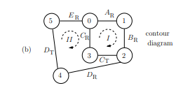
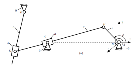
A planar mechanism is shown in Fig. 1.6a. The mechanism has five moving links $1,2,3,4,5$, and a fixed link, the ground 0 . The translation along the $i$ axis is denoted by $\mathrm{T}{i}$, and the rotation about the $i$ axis is denoted by $\mathrm{R}{i}$, where $i=x, y, z$. The motion of each link in the mechanism is analyzed in terms of its translation and rotation about the fixed reference frame $x y z$. The link 0 (ground) has no translations and no rotations. The link 1 has a rotation motion about the $z$ axis, $\mathrm{R}{z}$. The link 2 has a planar motion ( $x y$ is the plane of motion) with a translation along the $x$ axis, $\mathrm{T}{x}$, a translation along the $y$ axis, $\mathrm{T}{y}$, and a rotation about the $z$ axis, $\mathrm{R}{z}$. The link 3 (slider) has a rotation motion about the $z$ axis, $\mathrm{R}{z}$. The link 4 has a planar motion $(x y$ the plane of motion) with a translation along $x, \mathrm{~T}{x}$, a translation along $y, \mathrm{~T}{y}$, and a rotation about $z, \mathrm{R}{z}$. The link 5 has a rotation about the $z$ axis, $\mathrm{R}_{z}$.
A graphical construction for the mechanism connectivity is the contour diagram $[3,18]$. The numbered links are the nodes of the diagram and are represented by
circles, and the joints are represented by lines that connect the nodes. Figure $1.6 \mathrm{~b}$ is the contour diagram of the planar mechanism. The link 1 is connected to ground 0 at $A$ and to link 2 at $B$ with revolute joints. The link 2 is connected to link 3 at $C$ with a slider joint. The link 3 is connected to ground 0 at $C$ with a revolute joint. Next, the link 2 is connected to link 4 at $D$ with a revolute joint. Link 2 is a ternary link because it is connected to three links. Link 4 is connected to link 5 at $D$ with a slider joint. Link 5 is connected to ground 0 at $E$ with a revolute joint. The independent contour is the contour with at least one link that is not included in any other contours of the chain. The number of independent contours, $N$, of a kinematic chain is computed as
$$
N=c-n
$$
where $c$ is the number of joints, and $n$ is the number of moving links.
For the mechanism shown in Fig. 1.6a the independent contours are $N=c-n=$ $7-5=2$, where $c=7$ is the number of joints and $n=5$ is the number of moving links. Some contours of the mechanisms can be selected as: $0-1-2-3-0,0-1-2-4-5-0$, and 0-3-2-4-5-0. Only two contours are independent contours.
matlab代写
数学代写|matlab仿真代写simulation代做|Kinematic Pairs
连杆由连杆和关节组成,是机构和机器人的基本元件。链接(元素或成员)是具有节点的刚体。节点是可以连接链接的点。数字1.1显示具有两个节点的链接,即二元链接。具有三个节点的链接是三元链接。运动学副或关节是两个或多个连杆之间的连接。运动学对给出连接元素之间的相对运动。运动学副的自由度是建立连接链接相对位置的独立坐标的数量。
一个关节有(6−一世)自由度一世是限制相对运动的数量。平面一自由度运动副,C5, 去除 5 个自由度并允许 1 个自由度。平面二自由度运动副,C4, 有两个自由度,去掉 4 个自由度。为了找到运动学对的自由度,将一个元素保持为参考链接,并找到另一个元素相对于参考链接的位置。图 1.2a 显示了一个滑块(平移或棱柱)关节,它允许元素 1 和 2 之间的一个平移 (T) 自由度。1.2b表示允许连杆 1 和 2 之间有一个旋转 (R) 自由度的旋转销(旋转或旋转)关节。滑块和销接头是C5关节。这C5关节允许一个自由度,称为全关节。对于两个自由度关节,C4,在连接的链接之间有两个独立的相对运动,平移 (T) 和旋转 (R)。两个自由度关节如图 1.3 所示。两个自由度的关节称为半关节,有4个约束度。对于平面系统,有两种关节C5和C4. 操纵杆(球窝关节,或球形关节)是一个三自由度关节(3 个约束度,C3)并允许三个独立的运动。一个四自由度关节的例子,C2, 是平面上的圆柱体。五自由度关节,C1, 由平面上的球体表示。链接之间的接触可以是点、曲线或曲面。点或曲线接触定义了较高的关节,而曲面接触定义了较低的关节。关节的顺序定义为连接的链接数减一。两个连接的连杆的顺序为一(一个关节),三个连接的连杆的顺序为二(两个关节)。
数学代写|matlab仿真代写simulation代做|Degrees of Freedom
在任何时候唯一地定义机械系统在空间中位置的自变量的数量被定义为自由度(DOF)的数量。自由度的数量是关于参考系的。
数字1.4表示移动的刚体 (RB)X是-飞机。刚体上任意两个粒子之间的距离在任何时候都是恒定的。需要三个自由度来定义平面运动中自由刚体的位置:两个线性坐标(X,是)定义刚体上一点的位置,以及一个角坐标(θ)定义主体相对于参考轴的角度。确定其位置的独立测量的特定选择不是唯一的。在三维 (3-D) 空间中移动的自由刚体有六个自由度:三个长度(X,是,和), 和三个角(θX,θ是,θ和). 接下来只介绍二维运动。如果刚体具有相对于固定参考系没有运动的一点(旋转中心),则平面运动中的刚体具有纯旋转。身体上的点描述了相对于其中心的弧线。如果刚体上的所有点都描述平行路径,则平面运动中的刚体具有纯平移。平面运动中的刚体如果同时具有旋转和平移的组合,则它具有复杂或一般的平面运动。一般平面运动中身体上的点描述了在瞬时旋转中心处的非平行路径将改变其位置。
数学代写|matlab仿真代写simulation代做|Kinematic Chains
由关节连接的身体形成运动链,如图 1.5 所示。轮廓或环是由闭合的多边形链描述的配置,该链由由关节连接的链接组成,图 1.5a。闭合运动链具有结合在至少一个环中的每个链节和每个关节。图 1 闭环运动链1.5a 由链接定义0,1,2,3, 和 0 。图 1.5b 中的开放运动链由链接定义0,1,2, 和 3 . 机构是封闭的运动链。机器人是一个开放的运动链。混合运动链是闭合运动链和开放运动链的组合。曲柄是一个连杆,它围绕一个固定的枢轴旋转一圈。图 1.5a 中的链接 1 是曲柄。摇杆是一个带有振荡旋转的链接,固定在地面上。耦合器或连杆是具有复杂运动且不固定在地面上的连杆。图 2 中的链接1.5一种是一个耦合器。地面或固定框架是相对于参考框架固定(不动)的链接。地面用 0 表示。
平面机构如图 1.6a 所示。该机构有五个活动连杆1,2,3,4,5,和一个固定的链接,地面 0 。沿途的翻译一世轴表示为吨一世,以及围绕一世轴表示为R一世, 在哪里一世=X,是,和. 机构中每个连杆的运动都根据其围绕固定参考系的平移和旋转进行分析X是和. 链接 0(地面)没有平移和旋转。连杆 1 围绕和轴,R和. 连杆 2 具有平面运动 (X是是运动平面),沿X轴,吨X, 沿的翻译是轴,吨是,并围绕和轴,R和. 连杆 3(滑块)围绕和轴,R和. 连杆4具有平面运动(X是运动平面)沿平移X, 吨X, 翻译沿是, 吨是, 和一个关于和,R和. 连杆 5 围绕和轴,R和.
机构连通性的图形构造是等高线图[3,18]. 带编号的链接是图表的节点,由
圆,关节由连接节点的线表示。数字1.6 b是平面机构的轮廓图。链路 1 连接到地 0 在一种并将 2 链接到乙带有旋转关节。链路 2 连接到链路 3C带滑块接头。链路 3 连接到地 0 在C带旋转接头。接下来,链路 2 在以下位置连接到链路 4D带旋转接头。链路 2 是三元链路,因为它连接到三个链路。链路 4 连接到链路 5D带滑块接头。链路 5 连接到地 0 在和带旋转接头。独立轮廓是具有至少一个不包括在链的任何其他轮廓中的链节的轮廓。独立轮廓的数量,ñ, 运动链的计算为
ñ=C−n
在哪里C是关节的数量,并且n是移动链接的数量。
对于图 1.6a 所示的机制,独立轮廓为ñ=C−n= 7−5=2, 在哪里C=7是关节的数量和n=5是移动链接的数量。机构的一些轮廓可以选择为:0−1−2−3−0,0−1−2−4−5−0, 和 0-3-2-4-5-0。只有两个轮廓是独立的轮廓。

统计代写请认准statistics-lab™. statistics-lab™为您的留学生涯保驾护航。
金融工程代写
金融工程是使用数学技术来解决金融问题。金融工程使用计算机科学、统计学、经济学和应用数学领域的工具和知识来解决当前的金融问题,以及设计新的和创新的金融产品。
非参数统计代写
非参数统计指的是一种统计方法,其中不假设数据来自于由少数参数决定的规定模型;这种模型的例子包括正态分布模型和线性回归模型。
广义线性模型代考
广义线性模型(GLM)归属统计学领域,是一种应用灵活的线性回归模型。该模型允许因变量的偏差分布有除了正态分布之外的其它分布。
术语 广义线性模型(GLM)通常是指给定连续和/或分类预测因素的连续响应变量的常规线性回归模型。它包括多元线性回归,以及方差分析和方差分析(仅含固定效应)。
有限元方法代写
有限元方法(FEM)是一种流行的方法,用于数值解决工程和数学建模中出现的微分方程。典型的问题领域包括结构分析、传热、流体流动、质量运输和电磁势等传统领域。
有限元是一种通用的数值方法,用于解决两个或三个空间变量的偏微分方程(即一些边界值问题)。为了解决一个问题,有限元将一个大系统细分为更小、更简单的部分,称为有限元。这是通过在空间维度上的特定空间离散化来实现的,它是通过构建对象的网格来实现的:用于求解的数值域,它有有限数量的点。边界值问题的有限元方法表述最终导致一个代数方程组。该方法在域上对未知函数进行逼近。[1] 然后将模拟这些有限元的简单方程组合成一个更大的方程系统,以模拟整个问题。然后,有限元通过变化微积分使相关的误差函数最小化来逼近一个解决方案。
tatistics-lab作为专业的留学生服务机构,多年来已为美国、英国、加拿大、澳洲等留学热门地的学生提供专业的学术服务,包括但不限于Essay代写,Assignment代写,Dissertation代写,Report代写,小组作业代写,Proposal代写,Paper代写,Presentation代写,计算机作业代写,论文修改和润色,网课代做,exam代考等等。写作范围涵盖高中,本科,研究生等海外留学全阶段,辐射金融,经济学,会计学,审计学,管理学等全球99%专业科目。写作团队既有专业英语母语作者,也有海外名校硕博留学生,每位写作老师都拥有过硬的语言能力,专业的学科背景和学术写作经验。我们承诺100%原创,100%专业,100%准时,100%满意。
随机分析代写
随机微积分是数学的一个分支,对随机过程进行操作。它允许为随机过程的积分定义一个关于随机过程的一致的积分理论。这个领域是由日本数学家伊藤清在第二次世界大战期间创建并开始的。
时间序列分析代写
随机过程,是依赖于参数的一组随机变量的全体,参数通常是时间。 随机变量是随机现象的数量表现,其时间序列是一组按照时间发生先后顺序进行排列的数据点序列。通常一组时间序列的时间间隔为一恒定值(如1秒,5分钟,12小时,7天,1年),因此时间序列可以作为离散时间数据进行分析处理。研究时间序列数据的意义在于现实中,往往需要研究某个事物其随时间发展变化的规律。这就需要通过研究该事物过去发展的历史记录,以得到其自身发展的规律。
回归分析代写
多元回归分析渐进(Multiple Regression Analysis Asymptotics)属于计量经济学领域,主要是一种数学上的统计分析方法,可以分析复杂情况下各影响因素的数学关系,在自然科学、社会和经济学等多个领域内应用广泛。
MATLAB代写
MATLAB 是一种用于技术计算的高性能语言。它将计算、可视化和编程集成在一个易于使用的环境中,其中问题和解决方案以熟悉的数学符号表示。典型用途包括:数学和计算算法开发建模、仿真和原型制作数据分析、探索和可视化科学和工程图形应用程序开发,包括图形用户界面构建MATLAB 是一个交互式系统,其基本数据元素是一个不需要维度的数组。这使您可以解决许多技术计算问题,尤其是那些具有矩阵和向量公式的问题,而只需用 C 或 Fortran 等标量非交互式语言编写程序所需的时间的一小部分。MATLAB 名称代表矩阵实验室。MATLAB 最初的编写目的是提供对由 LINPACK 和 EISPACK 项目开发的矩阵软件的轻松访问,这两个项目共同代表了矩阵计算软件的最新技术。MATLAB 经过多年的发展,得到了许多用户的投入。在大学环境中,它是数学、工程和科学入门和高级课程的标准教学工具。在工业领域,MATLAB 是高效研究、开发和分析的首选工具。MATLAB 具有一系列称为工具箱的特定于应用程序的解决方案。对于大多数 MATLAB 用户来说非常重要,工具箱允许您学习和应用专业技术。工具箱是 MATLAB 函数(M 文件)的综合集合,可扩展 MATLAB 环境以解决特定类别的问题。可用工具箱的领域包括信号处理、控制系统、神经网络、模糊逻辑、小波、仿真等。