如果你也在 怎样代写SLAM这个学科遇到相关的难题,请随时右上角联系我们的24/7代写客服。
同步定位和测绘(SLAM)是构建或更新一个未知环境的地图,同时跟踪一个代理人在其中的位置的计算问题。虽然这最初似乎是一个鸡生蛋蛋生鸡的问题,但有几种已知的算法可以解决这个问题,至少是近似解决,在某些环境下是可行的。流行的近似解决方法包括粒子过滤器、扩展卡尔曼过滤器、协方差交叉和GraphSLAM。SLAM算法是基于计算几何和计算机视觉的概念,并被用于机器人导航、机器人测绘和虚拟现实或增强现实的里程测量。
statistics-lab™ 为您的留学生涯保驾护航 在代写SLAM方面已经树立了自己的口碑, 保证靠谱, 高质且原创的统计Statistics代写服务。我们的专家在代写SLAM代写方面经验极为丰富,各种代写SLAM相关的作业也就用不着说。
我们提供的SLAM及其相关学科的代写,服务范围广, 其中包括但不限于:
- Statistical Inference 统计推断
- Statistical Computing 统计计算
- Advanced Probability Theory 高等概率论
- Advanced Mathematical Statistics 高等数理统计学
- (Generalized) Linear Models 广义线性模型
- Statistical Machine Learning 统计机器学习
- Longitudinal Data Analysis 纵向数据分析
- Foundations of Data Science 数据科学基础
机器人代写|SLAM代写机器人导航代考|Adding New Landmarks
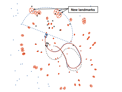
Adding a new landmark to FastSLAM can be difficult decision to make, just as with EKF-based algorithms. This is especially true when an individual measurement is insufficient to constrain the new landmark in all dimensions [13]. If the measurement function $g\left(\theta_{n_{t}}, s_{t}\right)$ is invertible, however, a single measurement is sufficient to initialize a new landmark. Each observation defines a Gaussian:
$$
\mathcal{N}\left(z_{t} ; \hat{z}{t}+G{\theta_{n_{t}}}\left(\theta_{n_{t}}-\mu_{n_{t}, t}^{[m]}\right), R_{t}\right)
$$
This Gaussian can be written explicitly as:
$$
\begin{aligned}
\frac{1}{\sqrt{\left|2 \pi R_{t}\right|}} \exp {&-\frac{1}{2}\left(z_{t}-\hat{z}{t}-G{\theta_{n_{t}}}\left(\theta_{n_{t}}-\mu_{n_{t}, t-1}^{[m]}\right)\right)^{T} \
&\left.R_{t}^{-1}\left(z_{t}-\hat{z}{t}-G{\theta_{n_{t}}}\left(\theta_{n_{t}}-\mu_{n_{t}, t-1}^{[m]}\right)\right)\right}
\end{aligned}
$$
We define a function J to be equal to the negative of the exponent of this Gaussian:
$$
J=\frac{1}{2}\left(z_{t}-\hat{z}{t}-G{\theta_{n_{t}}}\left(\theta_{n_{t}}-\mu_{n_{t}, t-1}^{[m]}\right)\right)^{T} R_{t}^{-1}\left(z_{t}-\hat{z}{t}-G{\theta_{n_{t}}}\left(\theta_{n_{t}}-\mu_{n_{t}, t-1}^{[m]}\right)\right)
$$
The second derivative of $J$ with respect to $\theta_{n_{t}}$ will be the inverse of the covariance matrix of the Gaussian in landmark coordinates.
$$
\begin{aligned}
\frac{\partial J}{\partial \theta_{n_{t}}} &=-\left(z_{t}-\hat{z}{t}-G{\theta_{n_{t}}}\left(\theta_{n_{t}}-\mu_{n_{t}, t-1}^{[m]}\right)\right)^{T} R_{t}^{-1} G_{\theta_{n_{t}}} \
\frac{\partial^{2} J}{\partial \theta_{n_{t}}^{2}} &=G_{\theta_{n_{t}}}^{T} R_{t}^{-1} G_{\theta_{n_{t}}}
\end{aligned}
$$
Consequently, an invertible observation can be used to create a new landmark as follows.
$$
\begin{aligned}
\mu_{n_{t}, t}^{[m]} &=g^{-1}\left(s_{t}^{[m]}, z_{t}\right) \
\Sigma_{n_{t}, t}^{[m]} &=\left(G_{\theta_{n_{t}}, t}^{T} R^{-1} G_{\theta_{n_{t}}, t}\right)^{-1} \
w_{t}^{[m]} &=p_{0}
\end{aligned}
$$
In practice, a simpler initialization procedure also works well. Instead of computing the correct initial covariance, the covariance can be computed by setting the variance of each landmark parameter to a large initial value $K$ and incorporating the first observation. Higher values of $K$ lead to closer approximations of the true covariance, but can also lead to numerical instability.
$$
\begin{aligned}
\mu_{n_{t}, t}^{[m]} &=g^{-1}\left(s_{t}^{[m]}, z_{t}\right) \
\Sigma_{n_{t}, t}^{[m]} &=K \cdot I
\end{aligned}
$$
Initialization techniques for situations in which $g$ is not invertible (e.g. bearings-only SLAM) are discussed in $[12,13]$. These situations require the accumulation of multiple observations in order to estimate the location of a landmark. FastSLAM is currently being applied to the problem of bearingsonly SLAM [83].
机器人代写|SLAM代写机器人导航代考|Summary of the FastSLAM Algorithm
Table $3.2$ summarizes the FastSLAM algorithm with unknown data association. Particles in the complete FastSLAM algorithm have the form:
$$
S_{t}^{[m]}=\left\langle s_{t}^{[m]} \mid N_{t}^{[m]}, \mu_{1, t}^{[m]}, \Sigma_{1, t}^{[m]}, \ldots, \mu_{N_{t}^{[m]}, t}^{[m]}, \Sigma_{N_{t}^{[m]}, t}^{[m]}\right\rangle
$$
In addition to the latest robot pose $s_{t}^{[m]}$ and the feature estimates $\mu_{n, t}^{[m]}$ and $\Sigma_{n, t}^{[m]}$, each particle maintains the number of features $N_{t}^{[m]}$ in its local map. It is interesting to note that each particle may have a different number of landmarks. This is an expressive representation, but it can lead to difficulties in determining the most probable map.
机器人代写|SLAM代写机器人导航代考|Greedy Mutual Exclusion
If multiple observations are incorporated simultaneously, the simplest approach to data association is to consider the identity of each observation independently. However, the data associations of each observation are clearly correlated, as was shown in Section 3.4. The data associations are correlated
through error in the robot pose, and they also must all obey a mutual exclusion constraint; more than one observation cannot be associated with the same landmark at the same time. Considering the data associations jointly does address these problems $[1,14,68]$, but these techniques are computationally expensive for large numbers of simultaneous observations.
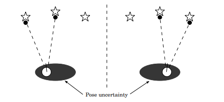
FastSLAM addresses the first problem, motion ambiguity, by sampling over robot poses and data associations. Each set of data association decisions is conditioned on a particular robot path. Thus, the data associations can be chosen independently without fear that pose error will corrupt all of the decisions. Some of the particles will chose the correct data associations, while others draw inconsistent robot poses, pick incorrect data associations, and receive low weights. Picking associations independently per particle still ignores the issue of mutual exclusion, however. Mutual exclusion is particularly useful for deciding when to add new landmarks in noisy environments. Instead of assigning an observation of an unseen landmark to an existing landmark, mutual exclusion will force the creation of a new landmark if both features are observed.
Proper handling of mutual exclusion requires that the data associations of all observations be considered simultaneously. However, mutual exclusion can also be enforced in a greedy fashion. Each observation is processed sequentially and ignores the landmarks associated with previously assigned observations. With a single data association hypothesis, applying mutual exclusion greedily can lead to failures in noisy environments. It can work well in FastSLAM, though, because the motion ambiguity that commonly causes greedy mutual exclusion failures is largely factored out by sampling over the the robot’s path. Furthermore, errors due to the greedy nature of the algorithm can also be minimized by processing the observations in different orders for each particle.
SLAM代写
机器人代写|SLAM代写机器人导航代考|Adding New Landmarks
与基于 EKF 的算法一样,向 FastSLAM 添加新的地标可能是一个艰难的决定。当单个测量不足以在所有维度上约束新地标时尤其如此 [13]。如果测量功能G(θn吨,s吨)是可逆的,然而,一次测量就足以初始化一个新的地标。每个观察定义一个高斯:
ñ(和吨;和^吨+Gθn吨(θn吨−μn吨,吨[米]),R吨)
这个高斯分布可以明确地写成:
\begin{aligned} \frac{1}{\sqrt{\left|2 \pi R_{t}\right|}} \exp {&-\frac{1}{2}\left(z_{t}- \hat{z}{t}-G{\theta_{n_{t}}}\left(\theta_{n_{t}}-\mu_{n_{t}, t-1}^{[m]} \right)\right)^{T} \ &\left.R_{t}^{-1}\left(z_{t}-\hat{z}{t}-G{\theta_{n_{t} }}\left(\theta_{n_{t}}-\mu_{n_{t}, t-1}^{[m]}\right)\right)\right} \end{aligned}\begin{aligned} \frac{1}{\sqrt{\left|2 \pi R_{t}\right|}} \exp {&-\frac{1}{2}\left(z_{t}- \hat{z}{t}-G{\theta_{n_{t}}}\left(\theta_{n_{t}}-\mu_{n_{t}, t-1}^{[m]} \right)\right)^{T} \ &\left.R_{t}^{-1}\left(z_{t}-\hat{z}{t}-G{\theta_{n_{t} }}\left(\theta_{n_{t}}-\mu_{n_{t}, t-1}^{[m]}\right)\right)\right} \end{aligned}
我们定义一个函数 J 等于这个高斯指数的负数:
Ĵ=12(和吨−和^吨−Gθn吨(θn吨−μn吨,吨−1[米]))吨R吨−1(和吨−和^吨−Gθn吨(θn吨−μn吨,吨−1[米]))
的二阶导数Ĵ关于θn吨将是高斯在地标坐标中的协方差矩阵的逆。
∂Ĵ∂θn吨=−(和吨−和^吨−Gθn吨(θn吨−μn吨,吨−1[米]))吨R吨−1Gθn吨 ∂2Ĵ∂θn吨2=Gθn吨吨R吨−1Gθn吨
因此,可以使用可逆观察来创建新的地标,如下所示。
μn吨,吨[米]=G−1(s吨[米],和吨) Σn吨,吨[米]=(Gθn吨,吨吨R−1Gθn吨,吨)−1 在吨[米]=p0
在实践中,更简单的初始化过程也可以很好地工作。可以通过将每个地标参数的方差设置为较大的初始值来计算协方差,而不是计算正确的初始协方差ķ并结合第一个观察结果。较高的值ķ导致更接近真实协方差,但也可能导致数值不稳定。
μn吨,吨[米]=G−1(s吨[米],和吨) Σn吨,吨[米]=ķ⋅一世
针对以下情况的初始化技术G是不可逆的(例如仅轴承 SLAM)在[12,13]. 这些情况需要累积多个观测值以估计地标的位置。FastSLAM 目前正在应用于仅轴承问题的 SLAM [83]。
机器人代写|SLAM代写机器人导航代考|Summary of the FastSLAM Algorithm
桌子3.2总结了未知数据关联的FastSLAM算法。完整的 FastSLAM 算法中的粒子具有以下形式:
小号吨[米]=⟨s吨[米]∣ñ吨[米],μ1,吨[米],Σ1,吨[米],…,μñ吨[米],吨[米],Σñ吨[米],吨[米]⟩
除了最新的机器人姿势s吨[米]和特征估计μn,吨[米]和Σn,吨[米],每个粒子保持特征的数量ñ吨[米]在其本地地图中。有趣的是,每个粒子可能有不同数量的界标。这是一种富有表现力的表示,但它可能会导致难以确定最可能的地图。
机器人代写|SLAM代写机器人导航代考|Greedy Mutual Exclusion
如果同时合并多个观察,最简单的数据关联方法是独立考虑每个观察的身份。然而,每个观察的数据关联显然是相关的,如第 3.4 节所示。数据关联是相关的
由于机器人姿态的错误,它们也必须都服从互斥约束;一个以上的观察不能同时与同一个地标相关联。联合考虑数据关联确实解决了这些问题[1,14,68],但这些技术对于大量同时观察的计算成本很高。
FastSLAM 通过对机器人姿势和数据关联进行采样来解决第一个问题,即运动模糊性。每组数据关联决策都以特定的机器人路径为条件。因此,可以独立选择数据关联,而不必担心姿势错误会破坏所有决策。一些粒子会选择正确的数据关联,而其他粒子会绘制不一致的机器人姿势,选择不正确的数据关联,并获得低权重。然而,每个粒子独立地选择关联仍然忽略了互斥问题。互斥对于决定何时在嘈杂环境中添加新地标特别有用。如果两个特征都被观察到,互斥将强制创建新的地标,而不是将未见地标的观察分配给现有地标。
正确处理互斥需要同时考虑所有观察值的数据关联。但是,互斥也可以以贪婪的方式强制执行。每个观察都按顺序处理,并忽略与先前分配的观察相关的界标。对于单一的数据关联假设,贪婪地应用互斥可能会导致在嘈杂环境中失败。不过,它可以在 FastSLAM 中很好地工作,因为通常会导致贪婪互斥失败的运动模糊性在很大程度上是通过对机器人路径的采样来排除的。此外,由于算法的贪心性质导致的错误也可以通过以不同顺序处理每个粒子的观察结果来最小化。

统计代写请认准statistics-lab™. statistics-lab™为您的留学生涯保驾护航。
金融工程代写
金融工程是使用数学技术来解决金融问题。金融工程使用计算机科学、统计学、经济学和应用数学领域的工具和知识来解决当前的金融问题,以及设计新的和创新的金融产品。
非参数统计代写
非参数统计指的是一种统计方法,其中不假设数据来自于由少数参数决定的规定模型;这种模型的例子包括正态分布模型和线性回归模型。
广义线性模型代考
广义线性模型(GLM)归属统计学领域,是一种应用灵活的线性回归模型。该模型允许因变量的偏差分布有除了正态分布之外的其它分布。
术语 广义线性模型(GLM)通常是指给定连续和/或分类预测因素的连续响应变量的常规线性回归模型。它包括多元线性回归,以及方差分析和方差分析(仅含固定效应)。
有限元方法代写
有限元方法(FEM)是一种流行的方法,用于数值解决工程和数学建模中出现的微分方程。典型的问题领域包括结构分析、传热、流体流动、质量运输和电磁势等传统领域。
有限元是一种通用的数值方法,用于解决两个或三个空间变量的偏微分方程(即一些边界值问题)。为了解决一个问题,有限元将一个大系统细分为更小、更简单的部分,称为有限元。这是通过在空间维度上的特定空间离散化来实现的,它是通过构建对象的网格来实现的:用于求解的数值域,它有有限数量的点。边界值问题的有限元方法表述最终导致一个代数方程组。该方法在域上对未知函数进行逼近。[1] 然后将模拟这些有限元的简单方程组合成一个更大的方程系统,以模拟整个问题。然后,有限元通过变化微积分使相关的误差函数最小化来逼近一个解决方案。
tatistics-lab作为专业的留学生服务机构,多年来已为美国、英国、加拿大、澳洲等留学热门地的学生提供专业的学术服务,包括但不限于Essay代写,Assignment代写,Dissertation代写,Report代写,小组作业代写,Proposal代写,Paper代写,Presentation代写,计算机作业代写,论文修改和润色,网课代做,exam代考等等。写作范围涵盖高中,本科,研究生等海外留学全阶段,辐射金融,经济学,会计学,审计学,管理学等全球99%专业科目。写作团队既有专业英语母语作者,也有海外名校硕博留学生,每位写作老师都拥有过硬的语言能力,专业的学科背景和学术写作经验。我们承诺100%原创,100%专业,100%准时,100%满意。
随机分析代写
随机微积分是数学的一个分支,对随机过程进行操作。它允许为随机过程的积分定义一个关于随机过程的一致的积分理论。这个领域是由日本数学家伊藤清在第二次世界大战期间创建并开始的。
时间序列分析代写
随机过程,是依赖于参数的一组随机变量的全体,参数通常是时间。 随机变量是随机现象的数量表现,其时间序列是一组按照时间发生先后顺序进行排列的数据点序列。通常一组时间序列的时间间隔为一恒定值(如1秒,5分钟,12小时,7天,1年),因此时间序列可以作为离散时间数据进行分析处理。研究时间序列数据的意义在于现实中,往往需要研究某个事物其随时间发展变化的规律。这就需要通过研究该事物过去发展的历史记录,以得到其自身发展的规律。
回归分析代写
多元回归分析渐进(Multiple Regression Analysis Asymptotics)属于计量经济学领域,主要是一种数学上的统计分析方法,可以分析复杂情况下各影响因素的数学关系,在自然科学、社会和经济学等多个领域内应用广泛。
MATLAB代写
MATLAB 是一种用于技术计算的高性能语言。它将计算、可视化和编程集成在一个易于使用的环境中,其中问题和解决方案以熟悉的数学符号表示。典型用途包括:数学和计算算法开发建模、仿真和原型制作数据分析、探索和可视化科学和工程图形应用程序开发,包括图形用户界面构建MATLAB 是一个交互式系统,其基本数据元素是一个不需要维度的数组。这使您可以解决许多技术计算问题,尤其是那些具有矩阵和向量公式的问题,而只需用 C 或 Fortran 等标量非交互式语言编写程序所需的时间的一小部分。MATLAB 名称代表矩阵实验室。MATLAB 最初的编写目的是提供对由 LINPACK 和 EISPACK 项目开发的矩阵软件的轻松访问,这两个项目共同代表了矩阵计算软件的最新技术。MATLAB 经过多年的发展,得到了许多用户的投入。在大学环境中,它是数学、工程和科学入门和高级课程的标准教学工具。在工业领域,MATLAB 是高效研究、开发和分析的首选工具。MATLAB 具有一系列称为工具箱的特定于应用程序的解决方案。对于大多数 MATLAB 用户来说非常重要,工具箱允许您学习和应用专业技术。工具箱是 MATLAB 函数(M 文件)的综合集合,可扩展 MATLAB 环境以解决特定类别的问题。可用工具箱的领域包括信号处理、控制系统、神经网络、模糊逻辑、小波、仿真等。