如果你也在 怎样代写SLAM这个学科遇到相关的难题,请随时右上角联系我们的24/7代写客服。
同步定位和测绘(SLAM)是构建或更新一个未知环境的地图,同时跟踪一个代理人在其中的位置的计算问题。虽然这最初似乎是一个鸡生蛋蛋生鸡的问题,但有几种已知的算法可以解决这个问题,至少是近似解决,在某些环境下是可行的。流行的近似解决方法包括粒子过滤器、扩展卡尔曼过滤器、协方差交叉和GraphSLAM。SLAM算法是基于计算几何和计算机视觉的概念,并被用于机器人导航、机器人测绘和虚拟现实或增强现实的里程测量。
statistics-lab™ 为您的留学生涯保驾护航 在代写SLAM方面已经树立了自己的口碑, 保证靠谱, 高质且原创的统计Statistics代写服务。我们的专家在代写SLAM代写方面经验极为丰富,各种代写SLAM相关的作业也就用不着说。
我们提供的SLAM及其相关学科的代写,服务范围广, 其中包括但不限于:
- Statistical Inference 统计推断
- Statistical Computing 统计计算
- Advanced Probability Theory 高等概率论
- Advanced Mathematical Statistics 高等数理统计学
- (Generalized) Linear Models 广义线性模型
- Statistical Machine Learning 统计机器学习
- Longitudinal Data Analysis 纵向数据分析
- Foundations of Data Science 数据科学基础
机器人代写|SLAM代写机器人导航代考|Proof of the FastSLAM Factorization
The FastSLAM factorization can be derived directly from the SLAM path posterior (3.2). Using the definition of conditional probability, the SLAM posterior can be rewritten as:
$$
p\left(s^{t}, \Theta \mid z^{t}, u^{t}, n^{t}\right)=p\left(s^{t} \mid z^{t}, u^{t}, n^{t}\right) p\left(\Theta \mid s^{t}, z^{t}, u^{t}, n^{t}\right)
$$
Thus, to derive the factored posterior (3.3), it suffices to show the following for all non-negative values of $t$ :
$$
p\left(\Theta \mid s^{t}, z^{t}, u^{t}, n^{t}\right)=\prod_{n=1}^{N} p\left(\theta_{n} \mid s^{t}, z^{t}, u^{t}, n^{t}\right)
$$
Proof of this statement can be demonstrated through induction. Two intermediate results must be derived in order to achieve this result. The first quantity to be derived is the probability of the observed landmark $\theta_{n_{t}}$ conditioned on the data. This quantity can be rewritten using Bayes Rule.
$$
p\left(\theta_{n_{t}} \mid s^{t}, z^{t}, u^{t}, n^{t}\right) \stackrel{\text { Bayes }}{=} \frac{p\left(z_{t} \mid \theta_{n_{t}}, s^{t}, z^{t-1}, u^{t}, n^{t}\right)}{p\left(z_{t} \mid s^{t}, z^{t-1}, u^{t}, n^{t}\right)} p\left(\theta_{n_{t}} \mid s^{t}, z^{t-1}, u^{t}, n^{t}\right)
$$
Note that the current observation $z_{t}$ depends solely on the current state of the robot and the landmark being observed. In the rightmost term of (3.6), we similarly notice that the current pose $s_{t}$, the current action $u_{t}$, and the current data association $n_{t}$ have no effect on $\theta_{n_{t}}$ without the current observation $z_{t}$. Thus, all of these variables can be dropped.
$$
p\left(\theta_{n_{t}} \mid s^{t}, z^{t}, u^{t}, n^{t}\right) \stackrel{M a r k o v}{=} \frac{p\left(z_{t} \mid \theta_{n_{t}}, s_{t}, n_{t}\right)}{p\left(z_{t} \mid s^{t}, z^{t-1}, u^{t}, n^{t}\right)} p\left(\theta_{n_{t}} \mid s^{t-1}, z^{t-1}, u^{t-1}, n^{t-1}\right)
$$
Next, we solve for the rightmost term of (3.7) to get:
$$
p\left(\theta_{n_{t}} \mid s^{t-1}, z^{t-1}, u^{t-1}, n^{t-1}\right)=\frac{p\left(z_{t} \mid s^{t}, z^{t-1}, u^{t}, n^{t}\right)}{p\left(z_{t} \mid \theta_{n_{t}}, s_{t}, n_{t}\right)} p\left(\theta_{n_{t}} \mid s^{t}, z^{t}, u^{t}, n^{t}\right)
$$
机器人代写|SLAM代写机器人导航代考|The FastSLAM 1.0 Algorithm
The factorization of the posterior (3.3) highlights important structure in the SLAM problem that is ignored by SLAM algorithms that estimate an unstructured posterior. This structure suggests that under the appropriate conditioning, no cross-correlations between landmarks have to be maintained explicitly. FastSLAM exploits the factored representation by maintaining $N+1$ filters, one for each term in (3.3). By doing so, all $N+1$ filters are low-dimensional.
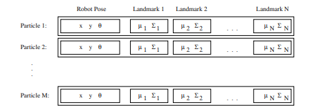
FastSLAM estimates the first term in (3.3), the robot path posterior, using a particle filter. The remaining $N$ conditional landmark posteriors $p\left(\theta_{n} \mid s^{t}, z^{t}, u^{t}, n^{t}\right)$ are estimated using EKFs. Each EKF tracks a single landmark position, and therefore is low-dimensional and fixed in size. The landmark EKFs are all conditioned on robot paths, with each particle in the particle filter possessing its own set of EKFs. In total, there are $N \cdot M$ EKFs, where $M$ is the total number of particles in the particle filter. The particle filter is depicted graphically in Figure 3.3. Each FastSLAM particle is of the form:
$$
S_{t}^{[m]}=\left\langle s^{t,[m]}, \mu_{1, t}^{[m]}, \Sigma_{1, t}^{[m]}, \ldots, \mu_{N, t}^{[m]}, \Sigma_{N, t}^{[m]}\right\rangle
$$
The bracketed notation $[m]$ indicates the index of the particle; $s^{t,[m]}$ is the $m$-th particle’s path estimate, and $\mu_{n, t}^{[m]}$ and $\Sigma_{n, t}^{[m]}$ are the mean and covariance of the Gaussian representing the $n$-th feature location conditioned on the path $s^{t,[m]}$. Together all of these quantities form the $m$-th particle $S_{t}^{[m]}$, of which there are a total of $M$ in the FastSLAM posterior. Filtering, that is, calculating the posterior at time $t$ from the one at time $t-1$, involves generating a new particle set $S_{t}$ from $S_{t-1}$, the particle set one time step earlier. The new particle set incorporates the latest control $u_{t}$ and measurement $z_{t}$ (with corresponding data association $n_{t}$ ). This update is performed in four steps.
First, a new robot pose is drawn for each particle that incorporates the latest control. Each pose is added to the appropriate robot path estimate $s^{t-1,[m]}$. Next, the landmark EKFs corresponding to the observed landmark are updated with the new observation. Since the robot path particles are not drawn from the true path posterior, each particle is given an importance weight to reflect this difference. A new set of particles $S_{t}$ is drawn from the weighted particle set using importance resampling. This importance resampling step is necessary to insure that the particles are distributed according to the true posterior (in the limit of infinite particles). The four basic steps of the FastSLAM algorithm $[59]$, shown in Table 3.1, will be explained in detail in the following four sections.
机器人代写|SLAM代写机器人导航代考|Sampling a New Pose
The particle set $S_{t}$ is calculated incrementally, from the set $S_{t-1}$ at time $t-1$, the observation $z_{t}$, and the control $u_{t}$. Since we cannot draw samples directly from the SLAM posterior at time $t$, we will instead draw samples from a simpler distribution called the proposal distribution, and correct for the difference using a technique called importance sampling.
In general, importance sampling is an algorithm for drawing samples from functions for which no direct sampling procedure exists [55]. Each sample drawn from the proposal distribution is given a weight equal to the ratio of the posterior distribution to the proposal distribution at that point in the sample space. A new set of unweighted samples is drawn from the weighted set with probabilities in proportion to the weights. This process is an instantiation of Rubin’s Sampling Importance Resampling (SIR) algorithm [79].
The proposal distribution of FastSLAM generate guesses of the robot’s pose at time $t$ given each particle $S_{t-1}^{[m]}$. This guess is obtained by sampling from the probabilistic motion model.
$$
s_{t}^{[m]} \sim p\left(s_{t} \mid u_{t}, s_{t-1}^{[m]}\right)
$$
This estimate is added to a temporary set of particles, along with the path $s^{t-1,[m]}$. Under the assumption that the set of particles $S_{t-1}$ is distributed according to $p\left(s^{t-1} \mid z^{t-1}, u^{t-1}, n^{t-1}\right)$, which is asymptotically correct, the new particles drawn from the proposal distribution are distributed according to:
$$
p\left(s^{t} \mid z^{t-1}, u^{t}, n^{t-1}\right)
$$
It is important to note that the motion model can be any non-linear function. This is in contrast to the EKF, which requires the motion model to be
linearized. The only practical limitation on the measurement model is that samples can be drawn from it conveniently. Regardless of the proposal distribution, drawing a new pose is a constant-time operation for every particle. It does not depend on the size of the map.
A simple four parameter motion model was used for all of the planar robot experiments in this book. This model assumes that the velocity of the robot is constant over the time interval covered by each control. Each control $u_{t}$ is two-dimensional and can be written as a translational velocity $v_{t}$ and a rotational velocity $\omega_{t}$. The model further assumes that the error in the controls is Gaussian. Note that this does not imply that error in the robot’s motion will also be Gaussian; the robot’s motion is a non-linear function of the controls and the control noise.
The errors in translational and rotational velocity have an additive and a multiplicative component. Throughout this book, the notation $\mathcal{N}(x ; \mu, \Sigma)$ will be used to denote a normal distribution over the variable $x$ with mean $\mu$ and covariance $\Sigma$.
$$
\begin{aligned}
v_{t}^{\prime} & \sim \mathcal{N}\left(v_{t}, \alpha_{1} v_{t}+\alpha_{2}\right) \
\omega_{t}^{\prime} & \sim \mathcal{N}\left(\omega_{t}, \alpha_{3} \omega_{t}+\alpha_{4}\right)
\end{aligned}
$$
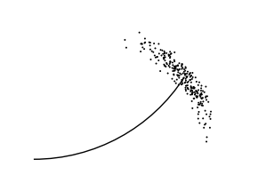
This motion model is able to represent the slip and skid errors errors that occur in typical ground vehicles [8]. The first step to drawing a new robot pose from this model is to draw a new translational and rotational velocity according to the observed control. The new pose $s_{t}$ can be calculated by simulating the new control forward from the previous pose $s_{t-1}^{[m]}$. Figure $3.4$ shows 250 samples drawn from this motion model given a curved trajectory. In this simulated example, the translational error of the robot is low, while the rotational error is high.
SLAM代写
机器人代写|SLAM代写机器人导航代考|Proof of the FastSLAM Factorization
FastSLAM 分解可以直接从 SLAM 路径后验 (3.2) 推导出来。使用条件概率的定义,SLAM 后验可以重写为:
p(s吨,θ∣和吨,在吨,n吨)=p(s吨∣和吨,在吨,n吨)p(θ∣s吨,和吨,在吨,n吨)
因此,要导出分解后的后验(3.3),对于所有非负值显示以下内容就足够了吨 :
p(θ∣s吨,和吨,在吨,n吨)=∏n=1ñp(θn∣s吨,和吨,在吨,n吨)
这个陈述的证明可以通过归纳来证明。为了达到这个结果,必须导出两个中间结果。要导出的第一个量是观察到的地标的概率θn吨以数据为条件。这个数量可以使用贝叶斯规则重写。
p(θn吨∣s吨,和吨,在吨,n吨)= 贝叶斯 p(和吨∣θn吨,s吨,和吨−1,在吨,n吨)p(和吨∣s吨,和吨−1,在吨,n吨)p(θn吨∣s吨,和吨−1,在吨,n吨)
注意当前观察和吨仅取决于机器人的当前状态和正在观察的地标。在 (3.6) 的最右边,我们同样注意到当前姿势s吨, 当前动作在吨,以及当前的数据关联n吨对没有影响θn吨没有当前的观察和吨. 因此,可以删除所有这些变量。
p(θn吨∣s吨,和吨,在吨,n吨)=米一种rķ这在p(和吨∣θn吨,s吨,n吨)p(和吨∣s吨,和吨−1,在吨,n吨)p(θn吨∣s吨−1,和吨−1,在吨−1,n吨−1)
接下来,我们求解 (3.7) 的最右边的项,得到:
p(θn吨∣s吨−1,和吨−1,在吨−1,n吨−1)=p(和吨∣s吨,和吨−1,在吨,n吨)p(和吨∣θn吨,s吨,n吨)p(θn吨∣s吨,和吨,在吨,n吨)
机器人代写|SLAM代写机器人导航代考|The FastSLAM 1.0 Algorithm
后验 (3.3) 的分解突出了 SLAM 问题中的重要结构,而估计非结构化后验的 SLAM 算法忽略了该结构。这种结构表明,在适当的条件下,地标之间的互相关性不必明确保持。FastSLAM 通过维护ñ+1过滤器,(3.3)中的每个术语一个。通过这样做,所有ñ+1过滤器是低维的。
FastSLAM 使用粒子滤波器估计 (3.3) 中的第一项,机器人路径后验。其余ñ条件地标后验p(θn∣s吨,和吨,在吨,n吨)使用 EKF 估计。每个 EKF 跟踪单个地标位置,因此是低维且大小固定的。地标 EKF 都以机器人路径为条件,粒子过滤器中的每个粒子都拥有自己的一组 EKF。总共有ñ⋅米EKF,其中米是粒子过滤器中的粒子总数。图 3.3 以图形方式描述了粒子过滤器。每个 FastSLAM 粒子的形式为:
小号吨[米]=⟨s吨,[米],μ1,吨[米],Σ1,吨[米],…,μñ,吨[米],Σñ,吨[米]⟩
括号内的符号[米]表示粒子的索引;s吨,[米]是个米-th 粒子的路径估计,和μn,吨[米]和Σn,吨[米]是表示高斯的均值和协方差n-th 以路径为条件的特征位置s吨,[米]. 所有这些量共同构成米-th 粒子小号吨[米], 其中一共有米在 FastSLAM 后验中。过滤,即计算时间的后验吨从那时起吨−1, 涉及生成一个新的粒子集小号吨从小号吨−1,粒子集提前了一个时间步。新的粒子集包含了最新的控制在吨和测量和吨(有相应的数据关联n吨)。此更新分四个步骤执行。
首先,为每个包含最新控制的粒子绘制一个新的机器人姿势。每个姿势都被添加到适当的机器人路径估计中s吨−1,[米]. 接下来,与观察到的界标相对应的界标 EKF 将使用新的观测值进行更新。由于机器人路径粒子不是从真实路径后验中提取的,因此每个粒子都被赋予了重要性权重以反映这种差异。一组新粒子小号吨是使用重要性重采样从加权粒子集中提取的。这个重要性重采样步骤对于确保粒子根据真实后验分布(在无限粒子的限制下)是必要的。FastSLAM算法的四个基本步骤[59],如表 3.1 所示,将在以下四节中详细说明。
机器人代写|SLAM代写机器人导航代考|Sampling a New Pose
粒子集小号吨增量计算,从集合小号吨−1有时吨−1, 观察和吨, 和控制在吨. 由于我们不能直接从 SLAM 后验中抽取样本吨,我们将改为从称为提议分布的更简单分布中抽取样本,并使用称为重要性采样的技术纠正差异。
一般来说,重要性抽样是一种从不存在直接抽样程序的函数中抽取样本的算法[55]。从提案分布中抽取的每个样本都被赋予一个权重,该权重等于样本空间中该点的后验分布与提案分布的比率。从加权集合中抽取一组新的未加权样本,概率与权重成正比。这个过程是鲁宾的采样重要性重采样(SIR)算法[79]的一个实例。
FastSLAM 的proposal distribution 对机器人的位姿进行猜测吨给定每个粒子小号吨−1[米]. 这个猜测是通过从概率运动模型中采样获得的。
s吨[米]∼p(s吨∣在吨,s吨−1[米])
该估计值与路径一起添加到一组临时粒子中s吨−1,[米]. 假设粒子集合小号吨−1根据分布p(s吨−1∣和吨−1,在吨−1,n吨−1),这是渐近正确的,从提议分布中抽取的新粒子的分布如下:
p(s吨∣和吨−1,在吨,n吨−1)
重要的是要注意运动模型可以是任何非线性函数。这与 EKF 形成对比,EKF 要求运动模型
线性化。测量模型的唯一实际限制是可以方便地从中抽取样本。无论提案分布如何,绘制一个新姿势对于每个粒子都是一个恒定时间的操作。它不依赖于地图的大小。
本书中的所有平面机器人实验都使用了一个简单的四参数运动模型。该模型假设机器人的速度在每个控制所覆盖的时间间隔内是恒定的。每个控件在吨是二维的,可以写成平移速度在吨和一个旋转速度ω吨. 该模型进一步假设控制中的误差是高斯的。请注意,这并不意味着机器人运动中的误差也会是高斯误差;机器人的运动是控制和控制噪声的非线性函数。
平移和旋转速度的误差具有加法和乘法分量。在本书中,符号ñ(X;μ,Σ)将用于表示变量的正态分布X平均μ和协方差Σ.
在吨′∼ñ(在吨,一种1在吨+一种2) ω吨′∼ñ(ω吨,一种3ω吨+一种4)
该运动模型能够表示典型地面车辆中发生的打滑和打滑误差[8]。从该模型中绘制新机器人姿态的第一步是根据观察到的控制绘制新的平移和旋转速度。新姿势s吨可以通过模拟从前一个姿势向前的新控制来计算s吨−1[米]. 数字3.4显示了从给定弯曲轨迹的运动模型中抽取的 250 个样本。在这个模拟示例中,机器人的平移误差较低,而旋转误差较高。

统计代写请认准statistics-lab™. statistics-lab™为您的留学生涯保驾护航。
金融工程代写
金融工程是使用数学技术来解决金融问题。金融工程使用计算机科学、统计学、经济学和应用数学领域的工具和知识来解决当前的金融问题,以及设计新的和创新的金融产品。
非参数统计代写
非参数统计指的是一种统计方法,其中不假设数据来自于由少数参数决定的规定模型;这种模型的例子包括正态分布模型和线性回归模型。
广义线性模型代考
广义线性模型(GLM)归属统计学领域,是一种应用灵活的线性回归模型。该模型允许因变量的偏差分布有除了正态分布之外的其它分布。
术语 广义线性模型(GLM)通常是指给定连续和/或分类预测因素的连续响应变量的常规线性回归模型。它包括多元线性回归,以及方差分析和方差分析(仅含固定效应)。
有限元方法代写
有限元方法(FEM)是一种流行的方法,用于数值解决工程和数学建模中出现的微分方程。典型的问题领域包括结构分析、传热、流体流动、质量运输和电磁势等传统领域。
有限元是一种通用的数值方法,用于解决两个或三个空间变量的偏微分方程(即一些边界值问题)。为了解决一个问题,有限元将一个大系统细分为更小、更简单的部分,称为有限元。这是通过在空间维度上的特定空间离散化来实现的,它是通过构建对象的网格来实现的:用于求解的数值域,它有有限数量的点。边界值问题的有限元方法表述最终导致一个代数方程组。该方法在域上对未知函数进行逼近。[1] 然后将模拟这些有限元的简单方程组合成一个更大的方程系统,以模拟整个问题。然后,有限元通过变化微积分使相关的误差函数最小化来逼近一个解决方案。
tatistics-lab作为专业的留学生服务机构,多年来已为美国、英国、加拿大、澳洲等留学热门地的学生提供专业的学术服务,包括但不限于Essay代写,Assignment代写,Dissertation代写,Report代写,小组作业代写,Proposal代写,Paper代写,Presentation代写,计算机作业代写,论文修改和润色,网课代做,exam代考等等。写作范围涵盖高中,本科,研究生等海外留学全阶段,辐射金融,经济学,会计学,审计学,管理学等全球99%专业科目。写作团队既有专业英语母语作者,也有海外名校硕博留学生,每位写作老师都拥有过硬的语言能力,专业的学科背景和学术写作经验。我们承诺100%原创,100%专业,100%准时,100%满意。
随机分析代写
随机微积分是数学的一个分支,对随机过程进行操作。它允许为随机过程的积分定义一个关于随机过程的一致的积分理论。这个领域是由日本数学家伊藤清在第二次世界大战期间创建并开始的。
时间序列分析代写
随机过程,是依赖于参数的一组随机变量的全体,参数通常是时间。 随机变量是随机现象的数量表现,其时间序列是一组按照时间发生先后顺序进行排列的数据点序列。通常一组时间序列的时间间隔为一恒定值(如1秒,5分钟,12小时,7天,1年),因此时间序列可以作为离散时间数据进行分析处理。研究时间序列数据的意义在于现实中,往往需要研究某个事物其随时间发展变化的规律。这就需要通过研究该事物过去发展的历史记录,以得到其自身发展的规律。
回归分析代写
多元回归分析渐进(Multiple Regression Analysis Asymptotics)属于计量经济学领域,主要是一种数学上的统计分析方法,可以分析复杂情况下各影响因素的数学关系,在自然科学、社会和经济学等多个领域内应用广泛。
MATLAB代写
MATLAB 是一种用于技术计算的高性能语言。它将计算、可视化和编程集成在一个易于使用的环境中,其中问题和解决方案以熟悉的数学符号表示。典型用途包括:数学和计算算法开发建模、仿真和原型制作数据分析、探索和可视化科学和工程图形应用程序开发,包括图形用户界面构建MATLAB 是一个交互式系统,其基本数据元素是一个不需要维度的数组。这使您可以解决许多技术计算问题,尤其是那些具有矩阵和向量公式的问题,而只需用 C 或 Fortran 等标量非交互式语言编写程序所需的时间的一小部分。MATLAB 名称代表矩阵实验室。MATLAB 最初的编写目的是提供对由 LINPACK 和 EISPACK 项目开发的矩阵软件的轻松访问,这两个项目共同代表了矩阵计算软件的最新技术。MATLAB 经过多年的发展,得到了许多用户的投入。在大学环境中,它是数学、工程和科学入门和高级课程的标准教学工具。在工业领域,MATLAB 是高效研究、开发和分析的首选工具。MATLAB 具有一系列称为工具箱的特定于应用程序的解决方案。对于大多数 MATLAB 用户来说非常重要,工具箱允许您学习和应用专业技术。工具箱是 MATLAB 函数(M 文件)的综合集合,可扩展 MATLAB 环境以解决特定类别的问题。可用工具箱的领域包括信号处理、控制系统、神经网络、模糊逻辑、小波、仿真等。