如果你也在 怎样代写监督学习Supervised and Unsupervised learning这个学科遇到相关的难题,请随时右上角联系我们的24/7代写客服。
监督学习算法从标记的训练数据中学习,帮你预测不可预见的数据的结果。成功地建立、扩展和部署准确的监督机器学习数据科学模型需要时间和高技能数据科学家团队的技术专长。此外,数据科学家必须重建模型,以确保给出的见解保持真实,直到其数据发生变化。
statistics-lab™ 为您的留学生涯保驾护航 在代写监督学习Supervised and Unsupervised learning方面已经树立了自己的口碑, 保证靠谱, 高质且原创的统计Statistics代写服务。我们的专家在代写监督学习Supervised and Unsupervised learning代写方面经验极为丰富,各种代写监督学习Supervised and Unsupervised learning相关的作业也就用不着说。
我们提供的监督学习Supervised and Unsupervised learning及其相关学科的代写,服务范围广, 其中包括但不限于:
- Statistical Inference 统计推断
- Statistical Computing 统计计算
- Advanced Probability Theory 高等概率论
- Advanced Mathematical Statistics 高等数理统计学
- (Generalized) Linear Models 广义线性模型
- Statistical Machine Learning 统计机器学习
- Longitudinal Data Analysis 纵向数据分析
- Foundations of Data Science 数据科学基础
机器学习代写|监督学习代考Supervised and Unsupervised learning代写|Linear Maximal Margin Classifier for Linearly Separable Data
Consider the problem of binary classification or dichotomization. Training data are given as
$$
\left(\mathbf{x}{1}, y\right),\left(\mathbf{x}{2}, y\right), \ldots,\left(\mathbf{x}{n}, y{n}\right), \mathbf{x} \in \Re^{m}, \quad y \in{+1,-1}
$$
For reasons of visualization only, we will consider the case of a two-dimensional input space, i.e., $\left(\mathbf{x} \in \Re^{2}\right)$. Data are linearly separable and there are many
different hyperplanes that can perform separation (Fig. 2.5). (Actually, for $\mathbf{x} \in \Re^{2}$, the separation is performed by ‘planes’ $w_{1} x_{1}+w_{2} x_{2}+b=d$. In other words, the decision boundary, i.e., the separation line in input space is defined by the equation $w_{1} x_{1}+w_{2} x_{2}+b=0$.). How to find ‘the best’ one? The difficult part is that all we have at our disposal are sparse training data. Thus, we want to find the optimal separating function without knowing the underlying probability distribution $P(\mathbf{x}, y)$. There are many functions that can solve given pattern recognition (or functional approximation) tasks. In such a problem setting, the SLT (developed in the early 1960 s by Vapnik and Chervonenkis [145]) shows that it is crucial to restrict the class of functions implemented by a learning machine to one with a complexity that is suitable for the amount of available training data.
In the case of a classification of linearly separable data, this idea is transformed into the following approach – among all the hyperplanes that minimize the training error (i.e., empirical risk) find the one with the largest margin. This is an intuitively acceptable approach. Just by looking at Fig $2.5$ we will find that the dashed separation line shown in the right graph seems to promise probably good classification while facing previously unseen data (meaning, in the generalization, i.e. test, phase). Or, at least, it seems to probably be better in generalization than the dashed decision boundary having smaller margin shown in the left graph. This can also be expressed as that a classifier with smaller margin will have higher expected risk. By using given training examples, during the learning stage, our machine finds parameters $\mathbf{w}=\left[\begin{array}{llll}w_{1} & w_{2} & \ldots & w_{m}\end{array}\right]^{T}$ and $b$ of a discriminant or decision function $d(\mathbf{x}, \mathbf{w}, b)$ given as
$$
d(\mathbf{x}, \mathbf{w}, b)=\mathbf{w}^{T} \mathbf{x}+b=\sum_{i=1}^{m} w_{i} x_{i}+b
$$
where $\mathbf{x}, \mathbf{w} \in \Re^{m}$, and the scalar $b$ is called a bias.(Note that the dashed separation lines in Fig. $2.5$ represent the line that follows from $d(\mathbf{x}, \mathbf{w}, b)=0)$. After the successful training stage, by using the weights obtained, the learning machine, given previously unseen pattern $\mathbf{x}{p}$, produces output $o$ according to an indicator function given as $$ i{F}=o=\operatorname{sign}\left(d\left(\mathbf{x}_{p}, \mathbf{w}, b\right)\right) .
$$
机器学习代写|监督学习代考Supervised and Unsupervised learning代写|Linear Soft Margin Classifier for Overlapping Classe
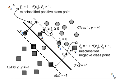
The learning procedure presented above is valid for linearly separable data, meaning for training data sets without overlapping. Such problems are rare in practice. At the same time, there are many instances when linear separating hyperplanes can be good solutions even when data are overlapped (e.g., normally distributed classes having the same covariance matrices have a linear separation boundary). However, quadratic programming solutions as given above cannot be used in the case of overlapping because the constraints $y_{i}\left[\mathbf{w}^{T} \mathbf{x}{i}+b\right] \geq 1, i=1, n$ given by (2.10b) cannot be satisfied. In the case of an overlapping (see Fig. 2.10), the overlapped data points cannot be correctly classified and for any misclassified training data point $\mathbf{x}{i}$, the corresponding $\alpha_{i}$ will tend to infinity. This particular data point (by increasing the corresponding $\alpha_{i}$ value) attempts to exert a stronger influence on the decision boundary in order to be classified correctly. When the $\alpha_{i}$ value reaches the maximal bound, it can no longer increase its effect, and the corresponding point will stay misclassified. In such a situation, the algorithm introduced above chooses all training data points as support vectors. To find a classifier with a maximal margin, the algorithm presented in the Sect. 2.2.1, must be changed allowing some data to be unclassified. Better to say, we must leave some data on the ‘wrong’ side of a decision boundary. In practice, we allow a soft margin and all data inside this margin (whether on the correct side of the separating line or on the wrong one) are neglected. The width of a soft margin can be controlled by a corresponding penalty parameter $C$ (introduced below) that determines the trade-off between the training error and VC dimension of the model.
The question now is how to measure the degree of misclassification and how to incorporate such a measure into the hard margin learning algorithm given by (2.10). The simplest method would be to form the following learning problem
$$
\min \frac{1}{2} \mathbf{w}^{T} \mathbf{w}+C \text { (number of misclassified data) }
$$
where $C$ is a penalty parameter, trading off the margin size (defined by $|\mathbf{w}|$, i.e., by $\mathbf{w}^{T} \mathbf{w}$ ) for the number of misclassified data points. Large $C$ leads to small number of misclassifications, bigger $\mathbf{w}^{T} \mathbf{w}$ and consequently to the smaller margin and vice versa. Obviously taking $C=\infty$ requires that the number of misclassified data is zero and, in the case of an overlapping this is not possible. Hence, the problem may be feasible only for some value $C<\infty$.
机器学习代写|监督学习代考Supervised and Unsupervised learning代写|The Nonlinear SVMs Classifier
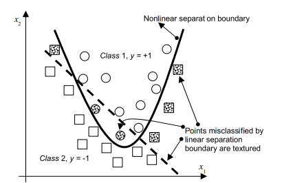
The linear classifiers presented in two previous sections are very limited. Mostly, classes are not only overlapped but the genuine separation functions are nonlinear hypersurfaces. A nice and strong characteristic of the approach presented above is that it can be easily (and in a relatively straightforward manner) extended to create nonlinear decision boundaries. The motivation for such an extension is that an SV machine that can create a nonlinear decision hypersurface will be able to classify nonlinearly separable data. This will be achieved by considering a linear classifier in the so-called feature space that will be introduced shortly. A very simple example of a need for designing nonlinear models is given in Fig. $2.11$ where the true separation boundary is quadratic. It is obvious that no errorless linear separating hyperplane can be found now. The best linear separation function shown as a dashed straight line would make six misclassifications (textured data points; 4 in the negative class and 2 in the positive one). Yet, if we use the nonlinear separation boundary we are able to separate two classes without any error. Generally, for $n$-dimensional input patterns, instead of a nonlinear curve, an SV machine will create a nonlinear separating hypersurface.
监督学习代写
机器学习代写|监督学习代考Supervised and Unsupervised learning代写|Linear Maximal Margin Classifier for Linearly Separable Data
考虑二元分类或二分法的问题。训练数据给出为
(X1,是),(X2,是),…,(Xn,是n),X∈ℜ米,是∈+1,−1
仅出于可视化的原因,我们将考虑二维输入空间的情况,即(X∈ℜ2). 数据是线性可分的,有很多
可以执行分离的不同超平面(图 2.5)。(实际上,对于X∈ℜ2, 分离由“平面”执行在1X1+在2X2+b=d. 换句话说,决策边界,即输入空间中的分隔线由等式定义在1X1+在2X2+b=0.)。如何找到“最好的”?困难的部分是我们可以使用的只是稀疏的训练数据。因此,我们希望在不知道潜在概率分布的情况下找到最优分离函数磷(X,是). 有许多函数可以解决给定的模式识别(或函数逼近)任务。在这样的问题设置中,SLT(由 Vapnik 和 Chervonenkis [145] 在 1960 年代初期开发)表明,将学习机实现的功能类别限制为具有适合数量的复杂性的功能至关重要可用的训练数据。
在线性可分数据分类的情况下,这个想法被转化为以下方法——在所有使训练误差(即经验风险)最小化的超平面中找到具有最大边际的超平面。这是一种直观可接受的方法。只看图2.5我们会发现,右图中显示的虚线分隔线似乎有望在面对以前看不见的数据时进行良好的分类(意思是泛化,即测试阶段)。或者,至少,它似乎比左图中显示的具有较小边距的虚线决策边界在泛化方面更好。这也可以表示为具有较小边际的分类器将具有较高的预期风险。通过使用给定的训练示例,在学习阶段,我们的机器找到参数在=[在1在2…在米]吨和b判别函数或决策函数d(X,在,b)给出为d(X,在,b)=在吨X+b=∑一世=1米在一世X一世+b
在哪里X,在∈ℜ米, 和标量b称为偏差。(请注意,图 2 中的虚线分隔线。2.5表示从d(X,在,b)=0). 在成功的训练阶段之后,通过使用获得的权重,学习机,给出以前看不见的模式Xp, 产生输出这根据给出的指示函数一世F=这=符号(d(Xp,在,b)).
机器学习代写|监督学习代考Supervised and Unsupervised learning代写|Linear Soft Margin Classifier for Overlapping Classe
上面介绍的学习过程适用于线性可分数据,这意味着训练数据集没有重叠。此类问题在实践中很少见。同时,在许多情况下,即使数据重叠(例如,具有相同协方差矩阵的正态分布类具有线性分离边界),线性分离超平面也可以成为很好的解决方案。然而,上面给出的二次规划解决方案不能在重叠的情况下使用,因为约束是一世[在吨X一世+b]≥1,一世=1,n(2.10b) 给出的不能满足。在重叠的情况下(见图 2.10),重叠的数据点无法正确分类,对于任何错误分类的训练数据点X一世, 相应的一种一世会趋于无穷大。这个特定的数据点(通过增加相应的一种一世value) 试图对决策边界施加更强的影响,以便正确分类。当。。。的时候一种一世值达到最大界限,就不能再增加效果,对应的点会一直误分类。在这种情况下,上面介绍的算法选择所有训练数据点作为支持向量。为了找到具有最大边距的分类器,Sect 中提出的算法。2.2.1,必须更改允许某些数据不分类。更好的说法是,我们必须在决策边界的“错误”一侧留下一些数据。在实践中,我们允许一个软边距,并且该边距内的所有数据(无论是在分隔线的正确一侧还是在错误的一侧)都将被忽略。软边距的宽度可以通过相应的惩罚参数来控制C(下文介绍)决定了模型的训练误差和 VC 维度之间的权衡。
现在的问题是如何衡量错误分类的程度,以及如何将这样的衡量标准纳入(2.10)给出的硬边距学习算法中。最简单的方法是形成以下学习问题
分钟12在吨在+C (错误分类数据的数量)
在哪里C是一个惩罚参数,权衡保证金大小(定义为|在|,即,由在吨在) 用于错误分类数据点的数量。大的C导致少量错误分类,更大在吨在从而导致较小的边距,反之亦然。显然采取C=∞要求错误分类数据的数量为零,并且在重叠的情况下这是不可能的。因此,该问题可能仅对某些值是可行的C<∞.
机器学习代写|监督学习代考Supervised and Unsupervised learning代写|The Nonlinear SVMs Classifier
前两节中介绍的线性分类器非常有限。大多数情况下,类不仅是重叠的,而且真正的分离函数是非线性超曲面。上述方法的一个很好且强大的特征是它可以很容易地(并且以相对直接的方式)扩展以创建非线性决策边界。这种扩展的动机是可以创建非线性决策超曲面的 SV 机器将能够对非线性可分数据进行分类。这将通过在即将介绍的所谓特征空间中考虑线性分类器来实现。图 1 给出了一个需要设计非线性模型的非常简单的例子。2.11其中真正的分离边界是二次的。很明显,现在找不到无误差的线性分离超平面。显示为虚线直线的最佳线性分离函数会产生 6 个错误分类(纹理数据点;4 个在负类中,2 个在正类中)。然而,如果我们使用非线性分离边界,我们就可以毫无错误地分离两个类别。一般来说,对于n维输入模式,而不是非线性曲线,SV 机器将创建非线性分离超曲面。

统计代写请认准statistics-lab™. statistics-lab™为您的留学生涯保驾护航。
金融工程代写
金融工程是使用数学技术来解决金融问题。金融工程使用计算机科学、统计学、经济学和应用数学领域的工具和知识来解决当前的金融问题,以及设计新的和创新的金融产品。
非参数统计代写
非参数统计指的是一种统计方法,其中不假设数据来自于由少数参数决定的规定模型;这种模型的例子包括正态分布模型和线性回归模型。
广义线性模型代考
广义线性模型(GLM)归属统计学领域,是一种应用灵活的线性回归模型。该模型允许因变量的偏差分布有除了正态分布之外的其它分布。
术语 广义线性模型(GLM)通常是指给定连续和/或分类预测因素的连续响应变量的常规线性回归模型。它包括多元线性回归,以及方差分析和方差分析(仅含固定效应)。
有限元方法代写
有限元方法(FEM)是一种流行的方法,用于数值解决工程和数学建模中出现的微分方程。典型的问题领域包括结构分析、传热、流体流动、质量运输和电磁势等传统领域。
有限元是一种通用的数值方法,用于解决两个或三个空间变量的偏微分方程(即一些边界值问题)。为了解决一个问题,有限元将一个大系统细分为更小、更简单的部分,称为有限元。这是通过在空间维度上的特定空间离散化来实现的,它是通过构建对象的网格来实现的:用于求解的数值域,它有有限数量的点。边界值问题的有限元方法表述最终导致一个代数方程组。该方法在域上对未知函数进行逼近。[1] 然后将模拟这些有限元的简单方程组合成一个更大的方程系统,以模拟整个问题。然后,有限元通过变化微积分使相关的误差函数最小化来逼近一个解决方案。
tatistics-lab作为专业的留学生服务机构,多年来已为美国、英国、加拿大、澳洲等留学热门地的学生提供专业的学术服务,包括但不限于Essay代写,Assignment代写,Dissertation代写,Report代写,小组作业代写,Proposal代写,Paper代写,Presentation代写,计算机作业代写,论文修改和润色,网课代做,exam代考等等。写作范围涵盖高中,本科,研究生等海外留学全阶段,辐射金融,经济学,会计学,审计学,管理学等全球99%专业科目。写作团队既有专业英语母语作者,也有海外名校硕博留学生,每位写作老师都拥有过硬的语言能力,专业的学科背景和学术写作经验。我们承诺100%原创,100%专业,100%准时,100%满意。
随机分析代写
随机微积分是数学的一个分支,对随机过程进行操作。它允许为随机过程的积分定义一个关于随机过程的一致的积分理论。这个领域是由日本数学家伊藤清在第二次世界大战期间创建并开始的。
时间序列分析代写
随机过程,是依赖于参数的一组随机变量的全体,参数通常是时间。 随机变量是随机现象的数量表现,其时间序列是一组按照时间发生先后顺序进行排列的数据点序列。通常一组时间序列的时间间隔为一恒定值(如1秒,5分钟,12小时,7天,1年),因此时间序列可以作为离散时间数据进行分析处理。研究时间序列数据的意义在于现实中,往往需要研究某个事物其随时间发展变化的规律。这就需要通过研究该事物过去发展的历史记录,以得到其自身发展的规律。
回归分析代写
多元回归分析渐进(Multiple Regression Analysis Asymptotics)属于计量经济学领域,主要是一种数学上的统计分析方法,可以分析复杂情况下各影响因素的数学关系,在自然科学、社会和经济学等多个领域内应用广泛。
MATLAB代写
MATLAB 是一种用于技术计算的高性能语言。它将计算、可视化和编程集成在一个易于使用的环境中,其中问题和解决方案以熟悉的数学符号表示。典型用途包括:数学和计算算法开发建模、仿真和原型制作数据分析、探索和可视化科学和工程图形应用程序开发,包括图形用户界面构建MATLAB 是一个交互式系统,其基本数据元素是一个不需要维度的数组。这使您可以解决许多技术计算问题,尤其是那些具有矩阵和向量公式的问题,而只需用 C 或 Fortran 等标量非交互式语言编写程序所需的时间的一小部分。MATLAB 名称代表矩阵实验室。MATLAB 最初的编写目的是提供对由 LINPACK 和 EISPACK 项目开发的矩阵软件的轻松访问,这两个项目共同代表了矩阵计算软件的最新技术。MATLAB 经过多年的发展,得到了许多用户的投入。在大学环境中,它是数学、工程和科学入门和高级课程的标准教学工具。在工业领域,MATLAB 是高效研究、开发和分析的首选工具。MATLAB 具有一系列称为工具箱的特定于应用程序的解决方案。对于大多数 MATLAB 用户来说非常重要,工具箱允许您学习和应用专业技术。工具箱是 MATLAB 函数(M 文件)的综合集合,可扩展 MATLAB 环境以解决特定类别的问题。可用工具箱的领域包括信号处理、控制系统、神经网络、模糊逻辑、小波、仿真等。