如果你也在 怎样代写理论力学Theoretical Mechanics这个学科遇到相关的难题,请随时右上角联系我们的24/7代写客服。
理论力学是研究物质的运动和导致这种运动的力量。它被应用于分析任何动态系统,从原子到太阳系。薄壁管的应力、变形和稳定性分析是物理学和工程学的一个经典课题。
statistics-lab™ 为您的留学生涯保驾护航 在代写理论力学Theoretical Mechanics方面已经树立了自己的口碑, 保证靠谱, 高质且原创的统计Statistics代写服务。我们的专家在代写理论力学Theoretical Mechanics代写方面经验极为丰富,各种代写理论力学Theoretical Mechanics相关的作业也就用不着说。
我们提供的理论力学Theoretical Mechanics及其相关学科的代写,服务范围广, 其中包括但不限于:
- Statistical Inference 统计推断
- Statistical Computing 统计计算
- Advanced Probability Theory 高等概率论
- Advanced Mathematical Statistics 高等数理统计学
- (Generalized) Linear Models 广义线性模型
- Statistical Machine Learning 统计机器学习
- Longitudinal Data Analysis 纵向数据分析
- Foundations of Data Science 数据科学基础
物理代写|理论力学作业代写Theoretical Mechanics代考|Notions
The technique of ‘differentiation’, which we discussed in the previous section, follows the scope of work:
given: $\quad y=f(x)$
finding: $\quad f^{\prime}(x)=\frac{d f}{d x}:$ ‘derivation’,
The reverse program, namely
given: $\quad f^{\prime}(x)=\frac{d f}{d x}$
finding: $\quad y=f(x)$
leads to the technique of ‘integration’. Consider for example
$$
f^{\prime}(x)=c=\text { const }
$$
then we remember according to (1.77) that
$$
y=f(x)=c \cdot x
$$
fulfills the condition $f^{\prime}(x)=c$.
Definition $F(x)$ is the ‘antiderivative (primitive function)’ of $f(x)$, if it holds:
$$
F^{\prime}(x)=f(x) \quad \forall x
$$
In this connection the above example means:
$$
f(x) \equiv c \quad \curvearrowright \quad F(x)=c \cdot x+d .
$$
Because of the constant $d$ the result comes out as a full family of curves. Fixing $d$ needs the introduction of ‘boundary conditions’. We accept that:
‘Integration’ : Searching for the antiderivative (primitive function)
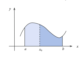
To generate a graphic image, the integral can be interpreted as the area under the curve $y=f(x)$. If the curve $y=f(x)$ is given then we ask ourselves how we can determine the area $F$ in Fig. $1.18$ under the curve between the limits $x=$ $a$ and $x=b$. This can easily be done for the special case that $f(x)$ represents a straight line. However, how can we calculate the area under an arbitrary (continuous) function $f(x)$ ?
In a first step, we approach the calculation of the area by decomposing the interval $[a, b]$ in $n$ equal sub-intervals $\Delta x_{n}$,
$$
\Delta x_{n}=\frac{b-a}{n} \quad n \in \mathbb{N} / 0
$$
where $x_{i}$ is the center of the $i$-th partial interval:
$$
x_{i}=a+\left(i-\frac{1}{2}\right) \Delta x_{n} ; i=1,2 \ldots, n
$$
Then $f\left(x_{i}\right) \Delta x_{n}$ is the area of the $i$-th pillar in Fig. 1.19. Hence it holds approximately for the area $F$ :
$$
F \approx \sum_{i=1}^{n} f\left(x_{i}\right) \Delta x_{n}
$$
物理代写|理论力学作业代写Theoretical Mechanics代考|First Rules of Integration
Some important rules follow directly from the definition of the integral:
- Identical bounds of integration:
$$
\int_{a}^{a} f(x) d x=0
$$ - The ‘area’ in the sense of an integral has a sign because of $f(x)<^{\geq}$! For the example in Fig. $1.20$ one recognizes: $$ \begin{aligned} &F_{1}=\int_{a}^{x_{1}} f(x) d x>0 \
&F_{2}=\int_{x_{1}}^{x_{2}} f(x) d x<0 \\ &F_{3}=\int_{x_{2}}^{x_{3}} f(x) d x>0
\end{aligned}
$$Constant factor $c \in \mathbb{R}$ : - $$
- \int_{a}^{b} c \cdot f(x) d x=\lim {n \rightarrow \infty} \sum{i=1}^{n} c \cdot f\left(x_{i}\right) \Delta x_{n}=c \cdot \lim {n \rightarrow \infty} \sum{i=1}^{n} f\left(x_{i}\right) \Delta x_{n}
- $$
- Hence it holds:
- $$
- \int_{a}^{b} c \cdot f(x) d x=c \cdot \int_{a}^{b} f(x) d x
- $$
- Sum:
- Assume
- $$
- f(x) \equiv g(x)+h(x)
- $$
- then it follows from the definition of the Riemann integral:
- $$
- \begin{aligned}
- \int_{a}^{b} f(x) d x &=\lim {n \rightarrow \infty} \sum{i=1}^{n}\left(g\left(x_{i}\right)+h\left(x_{i}\right)\right) \Delta x_{n} \
- &=\lim {n \rightarrow \infty} \sum{i=1}^{n} g\left(x_{i}\right) \Delta x_{n}+\lim {n \rightarrow \infty} \sum{i=1}^{n} h\left(x_{i}\right) \Delta x_{n}
- \end{aligned}
- $$
- That means:
- $$
- \int_{a}^{b} f(x) d x=\int_{a}^{b} g(x) d x+\int_{a}^{b} h(x) d x
- $$
- The last two rules of integration (1.112) and (1.113) demonstrate the linearity of the integral.
- Partitioning the interval of integration:
- $$
- \Delta x_{n}=\frac{b-a}{n}=\Delta x_{n}^{(1)}+\Delta x_{n}^{(2)}=\frac{x_{0}-a}{n}+\frac{b-x_{0}}{n}
- $$
- Therewith we can write:
- $$
- \int_{a}^{b} f(x) d x=\lim {n \rightarrow \infty} \sum{i=1}^{n} f\left(x_{i}^{(1)}\right) \Delta x_{n}^{(1)}+\lim {n \rightarrow \infty} \sum{i=1}^{n} f\left(x_{i}^{(2)}\right) \Delta x_{n}^{(2)}
- $$
物理代写|理论力学作业代写Theoretical Mechanics代考|Fundamental Theorem of Calculus
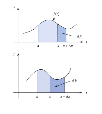
We consider the definite integral over a continuous function $f(t)$, but now with variable upper limit:
$$
F(x)=\int_{a}^{x} f(t) d t
$$
‘area function’
The area under the curve $f(t)$ in this case is not constant but a function of $x$ (Fig. 1.22). If the upper bound of integration is shifted by $\Delta x$ the area will change by:
$$
\Delta F=F(x+\Delta x)-F(x)=\int_{a}^{x+\Delta x} f(t) d t-\int_{a}^{x} f(t) d t=\int_{x}^{x+\Delta x} f(t) d t
$$
In the last step we have used the rule (1.114). Without explicit proof we accept the important
‘mean value theorem of integral calculus’
This theorem implies:
$$
\exists \hat{x} \in[x, x+\Delta x] \text { with } \Delta F=\Delta x \cdot f(\hat{x}) \text {. }
$$
Although not exactly proven the theorem appears rather plausible according to Fig. 1.23. So we can further conclude:
$$
F^{\prime}(x)=\lim {\Delta x \rightarrow 0} \frac{\Delta F}{\Delta x}=\lim {\Delta x \rightarrow 0} f(\hat{x})=f(x)
$$
Thus after $(1.105)$, the area function is the antiderivative of $f(x)$ ! Furthermore, the equivalence of the definitions $(1.105)$ and $(1.110)$ for the antiderivative, which
remained unsettled in Sect. 1.2.1, is now settled.
‘fundamental theorem of calculus’
$$
\frac{d}{d x} F(x) \equiv \frac{d}{d x} \int_{a}^{x} f(t) d t=f(x) .
$$
The successive performing of integration and differentiation obviously cancel each other!
$$
\text { integration } \cong \text { inversion of differentiation }
$$
The influence of the lower limit of integration in (1.118) still appears unsettled (Fig. 1.24). To clarify this we therefore investigate:
$$
\tilde{F}(x)=\int_{a^{\prime}}^{x} f(t) d t=\underbrace{\int_{a^{\prime}}^{a} f(t) d t}{=A, \text { independent of } x}+\underbrace{\int{a}^{x} f(t) d t}_{F(x)} .
$$
Therewith it follows that both $F(x)$ and $\tilde{F}(x)$ are antiderivatives of $f(x)$ :
$$
\tilde{F}(x)=F(x)+A \curvearrowright \frac{d}{d x} \tilde{F}(x)=\frac{d}{d x} F(x)=f(x) .
$$
The lower limit of integration is therefore in a certain sense dummy, the antiderivative is uniquely fixed except for an additive constant:
$$
F(x) \Longleftrightarrow \tilde{F}(x)=F(x)+A .
$$
Therefore one introduces the
$$
\text { ‘indefinite integral’: } \quad F(x)=\int f(x) d x \text {. }
$$
defining therewith the set of all antiderivatives of $f(x)$ !
理论力学代写
物理代写|理论力学作业代写Theoretical Mechanics代考|Notions
我们在上一节中讨论的“微分”技术遵循工作范围:
给定:是=F(X)
发现:F′(X)=dFdX:’derivation’,
逆向程序,即
给出:F′(X)=dFdX
发现:是=F(X)
导致“整合”技术。考虑例如
F′(X)=C= 常量
然后我们记得根据(1.77)
是=F(X)=C⋅X
满足条件F′(X)=C.
定义F(X)是’反导数(原始函数)’F(X),如果它成立:
F′(X)=F(X)∀X
在这方面,上面的例子意味着:
F(X)≡C↷F(X)=C⋅X+d.
因为不断d结果是一个完整的曲线族。定影d需要引入“边界条件”。我们接受:
“积分”:搜索反导数(原始函数)
要生成图形图像,积分可以解释为曲线下的面积是=F(X). 如果曲线是=F(X)给出然后我们问自己我们如何确定该区域F在图。1.18在界限之间的曲线下X= 一种和X=b. 对于以下特殊情况,这可以很容易地完成F(X)代表一条直线。但是,我们如何计算任意(连续)函数下的面积F(X) ?
第一步,我们通过分解区间来计算面积[一种,b]在n相等的子区间ΔXn,
ΔXn=b−一种nn∈ñ/0
在哪里X一世是中心一世-第部分间隔:
X一世=一种+(一世−12)ΔXn;一世=1,2…,n
然后F(X一世)ΔXn是面积一世-图 1.19 中的第一个支柱。因此,它大约适用于该地区F :
F≈∑一世=1nF(X一世)ΔXn
物理代写|理论力学作业代写Theoretical Mechanics代考|First Rules of Integration
一些重要的规则直接来自积分的定义:
- 相同的积分界限:
∫一种一种F(X)dX=0 - 积分意义上的“面积”有一个符号,因为F(X)<≥!对于图中的示例。1.20一个人承认:F1=∫一种X1F(X)dX>0 F2=∫X1X2F(X)dX<0F3=∫X2X3F(X)dX>0常数因子C∈R:
- $$
- \int_{a}^{b} c \cdot f(x) dx=\lim {n \rightarrow \infty} \sum{i=1}^{n} c \cdot f\left(x_{i}\右) \Delta x_{n}=c \cdot \lim {n \rightarrow \infty} \sum{i=1}^{n} f\left(x_{i}\right) \Delta x_{n}
- $$
- 因此它成立:
- $$
- \int_{a}^{b} c \cdot f(x) dx=c \cdot \int_{a}^{b} f(x) dx
- $$
- 和:
- 认为
- $$
- f(x) \equiv g(x)+h(x)
- $$
- 则由黎曼积分的定义得出:
- $$
- \开始{对齐}
- \int_{a}^{b} f(x) dx &=\lim {n \rightarrow \infty} \sum{i=1}^{n}\left(g\left(x_{i}\right) +h\left(x_{i}\right)\right) \Delta x_{n} \
- &=\lim {n \rightarrow \infty} \sum{i=1}^{n} g\left(x_{i}\right) \Delta x_{n}+\lim {n \rightarrow \infty} \ sum{i=1}^{n} h\left(x_{i}\right) \Delta x_{n}
- \end{对齐}
- $$
- 这意味着:
- $$
- \int_{a}^{b} f(x) dx=\int_{a}^{b} g(x) d x+\int_{a}^{b} h(x) dx
- $$
- 最后两个积分规则 (1.112) 和 (1.113) 证明了积分的线性。
- 划分积分区间:
- $$
- \Delta x_{n}=\frac{ba}{n}=\Delta x_{n}^{(1)}+\Delta x_{n}^{(2)}=\frac{x_{0}- a}{n}+\frac{b-x_{0}}{n}
- $$
- 我们可以这样写:
- $$
- \int_{a}^{b} f(x) dx=\lim {n \rightarrow \infty} \sum{i=1}^{n} f\left(x_{i}^{(1)}\右) \Delta x_{n}^{(1)}+\lim {n \rightarrow \infty} \sum{i=1}^{n} f\left(x_{i}^{(2)}\右)\Delta x_{n}^{(2)}
- $$
物理代写|理论力学作业代写Theoretical Mechanics代考|Fundamental Theorem of Calculus
我们考虑连续函数上的定积分F(吨),但现在有可变上限:
F(X)=∫一种XF(吨)d吨
‘面积函数’
曲线下面积F(吨)在这种情况下不是恒定的,而是一个函数X(图 1.22)。如果积分的上限移动了ΔX该区域将发生以下变化:
ΔF=F(X+ΔX)−F(X)=∫一种X+ΔXF(吨)d吨−∫一种XF(吨)d吨=∫XX+ΔXF(吨)d吨
在最后一步中,我们使用了规则 (1.114)。在没有明确证明的情况下,我们接受重要
的“积分中值定理”
这个定理意味着:
∃X^∈[X,X+ΔX] 和 ΔF=ΔX⋅F(X^).
根据图 1.23,虽然没有完全证明,但该定理似乎相当合理。所以我们可以进一步得出结论:
F′(X)=林ΔX→0ΔFΔX=林ΔX→0F(X^)=F(X)
因此之后(1.105), 面积函数是F(X)!此外,定义的等价性(1.105)和(1.110)对于反衍生物,它
在宗门里一直不安。1.2.1,现已解决。
‘微积分基本定理’
ddXF(X)≡ddX∫一种XF(吨)d吨=F(X).
整合与分化的先后进行,显然是相互抵消的!
一体化 ≅ 微分反转
The influence of the lower limit of integration in (1.118) still appears unsettled (Fig. 1.24). To clarify this we therefore investigate:
$$
\tilde{F}(x)=\int_{a^{\prime}}^{x} f(t) d t=\underbrace{\int_{a^{\prime}}^{a} f(t) d t}{=A, \text { independent of } x}+\underbrace{\int{a}^{x} f(t) d t}_{F(x)} .
Therewithitfollowsthatboth$F(x)$and$F~(x)$areantiderivativesof$f(x)$:
\tilde{F}(x)=F(x)+A \curvearrowright \frac{d}{d x} \tilde{F}(x)=\frac{d}{d x} F(x)=f(x) .
Thelowerlimitofintegrationisthereforeinacertainsensedummy,theantiderivativeisuniquelyfixedexceptforanadditiveconstant:
F(x) \Longleftrightarrow \tilde{F}(x)=F(x)+A .
Thereforeoneintroducesthe
\text { ‘indefinite integral’: } \quad F(x)=\int f(x) d x \text {. }
$$
defining therewith the set of all antiderivatives of f(x) !

统计代写请认准statistics-lab™. statistics-lab™为您的留学生涯保驾护航。
金融工程代写
金融工程是使用数学技术来解决金融问题。金融工程使用计算机科学、统计学、经济学和应用数学领域的工具和知识来解决当前的金融问题,以及设计新的和创新的金融产品。
非参数统计代写
非参数统计指的是一种统计方法,其中不假设数据来自于由少数参数决定的规定模型;这种模型的例子包括正态分布模型和线性回归模型。
广义线性模型代考
广义线性模型(GLM)归属统计学领域,是一种应用灵活的线性回归模型。该模型允许因变量的偏差分布有除了正态分布之外的其它分布。
术语 广义线性模型(GLM)通常是指给定连续和/或分类预测因素的连续响应变量的常规线性回归模型。它包括多元线性回归,以及方差分析和方差分析(仅含固定效应)。
有限元方法代写
有限元方法(FEM)是一种流行的方法,用于数值解决工程和数学建模中出现的微分方程。典型的问题领域包括结构分析、传热、流体流动、质量运输和电磁势等传统领域。
有限元是一种通用的数值方法,用于解决两个或三个空间变量的偏微分方程(即一些边界值问题)。为了解决一个问题,有限元将一个大系统细分为更小、更简单的部分,称为有限元。这是通过在空间维度上的特定空间离散化来实现的,它是通过构建对象的网格来实现的:用于求解的数值域,它有有限数量的点。边界值问题的有限元方法表述最终导致一个代数方程组。该方法在域上对未知函数进行逼近。[1] 然后将模拟这些有限元的简单方程组合成一个更大的方程系统,以模拟整个问题。然后,有限元通过变化微积分使相关的误差函数最小化来逼近一个解决方案。
tatistics-lab作为专业的留学生服务机构,多年来已为美国、英国、加拿大、澳洲等留学热门地的学生提供专业的学术服务,包括但不限于Essay代写,Assignment代写,Dissertation代写,Report代写,小组作业代写,Proposal代写,Paper代写,Presentation代写,计算机作业代写,论文修改和润色,网课代做,exam代考等等。写作范围涵盖高中,本科,研究生等海外留学全阶段,辐射金融,经济学,会计学,审计学,管理学等全球99%专业科目。写作团队既有专业英语母语作者,也有海外名校硕博留学生,每位写作老师都拥有过硬的语言能力,专业的学科背景和学术写作经验。我们承诺100%原创,100%专业,100%准时,100%满意。
随机分析代写
随机微积分是数学的一个分支,对随机过程进行操作。它允许为随机过程的积分定义一个关于随机过程的一致的积分理论。这个领域是由日本数学家伊藤清在第二次世界大战期间创建并开始的。
时间序列分析代写
随机过程,是依赖于参数的一组随机变量的全体,参数通常是时间。 随机变量是随机现象的数量表现,其时间序列是一组按照时间发生先后顺序进行排列的数据点序列。通常一组时间序列的时间间隔为一恒定值(如1秒,5分钟,12小时,7天,1年),因此时间序列可以作为离散时间数据进行分析处理。研究时间序列数据的意义在于现实中,往往需要研究某个事物其随时间发展变化的规律。这就需要通过研究该事物过去发展的历史记录,以得到其自身发展的规律。
回归分析代写
多元回归分析渐进(Multiple Regression Analysis Asymptotics)属于计量经济学领域,主要是一种数学上的统计分析方法,可以分析复杂情况下各影响因素的数学关系,在自然科学、社会和经济学等多个领域内应用广泛。
MATLAB代写
MATLAB 是一种用于技术计算的高性能语言。它将计算、可视化和编程集成在一个易于使用的环境中,其中问题和解决方案以熟悉的数学符号表示。典型用途包括:数学和计算算法开发建模、仿真和原型制作数据分析、探索和可视化科学和工程图形应用程序开发,包括图形用户界面构建MATLAB 是一个交互式系统,其基本数据元素是一个不需要维度的数组。这使您可以解决许多技术计算问题,尤其是那些具有矩阵和向量公式的问题,而只需用 C 或 Fortran 等标量非交互式语言编写程序所需的时间的一小部分。MATLAB 名称代表矩阵实验室。MATLAB 最初的编写目的是提供对由 LINPACK 和 EISPACK 项目开发的矩阵软件的轻松访问,这两个项目共同代表了矩阵计算软件的最新技术。MATLAB 经过多年的发展,得到了许多用户的投入。在大学环境中,它是数学、工程和科学入门和高级课程的标准教学工具。在工业领域,MATLAB 是高效研究、开发和分析的首选工具。MATLAB 具有一系列称为工具箱的特定于应用程序的解决方案。对于大多数 MATLAB 用户来说非常重要,工具箱允许您学习和应用专业技术。工具箱是 MATLAB 函数(M 文件)的综合集合,可扩展 MATLAB 环境以解决特定类别的问题。可用工具箱的领域包括信号处理、控制系统、神经网络、模糊逻辑、小波、仿真等。