如果你也在 怎样代写理论力学Theoretical Mechanics这个学科遇到相关的难题,请随时右上角联系我们的24/7代写客服。
理论力学是研究物质的运动和导致这种运动的力量。它被应用于分析任何动态系统,从原子到太阳系。薄壁管的应力、变形和稳定性分析是物理学和工程学的一个经典课题。
statistics-lab™ 为您的留学生涯保驾护航 在代写理论力学Theoretical Mechanics方面已经树立了自己的口碑, 保证靠谱, 高质且原创的统计Statistics代写服务。我们的专家在代写理论力学Theoretical Mechanics代写方面经验极为丰富,各种代写理论力学Theoretical Mechanics相关的作业也就用不着说。
我们提供的理论力学Theoretical Mechanics及其相关学科的代写,服务范围广, 其中包括但不限于:
- Statistical Inference 统计推断
- Statistical Computing 统计计算
- Advanced Probability Theory 高等概率论
- Advanced Mathematical Statistics 高等数理统计学
- (Generalized) Linear Models 广义线性模型
- Statistical Machine Learning 统计机器学习
- Longitudinal Data Analysis 纵向数据分析
- Foundations of Data Science 数据科学基础
物理代写|理论力学作业代写Theoretical Mechanics代考|Velocity and Acceleration
The motion of a mass point is characterized by:
position vector: $\mathbf{r}(t)$,
velocity vector: $\quad \mathbf{v}(t)=\dot{\mathbf{r}}(t)$.
acceleration vector: $\mathbf{a}(t)=\ddot{\mathbf{r}}(t)$.
Higher time derivatives do not interest us in mechanics; very often they even fail to exist because in many realistic cases the acceleration is not a continuous function of time.
The typical task for mechanics consists of the calculation of the path line (trajectory) $\mathbf{r}(t)$ on the basis of a given acceleration $\mathbf{a}(t)=\ddot{\mathbf{r}}(t)$. For this purpose one has obviously to integrate $\mathbf{a}(t)$ twice with respect to time. After each integration an integration constant appears which remains undetermined unless we have two initial conditions at our disposal to fix these constants. In this connection let us assume that we know the velocity and the position of the mass point (particle) at a certain time $t_{0}$, i.e.
$$
\mathbf{a}(t) \text { for all } t, \mathbf{v}\left(t_{0}\right) \text {, and } \mathbf{r}\left(t_{0}\right)
$$
are given. Then the velocity of the particle is determined by
$$
\mathbf{v}(t)=\mathbf{v}\left(t_{0}\right)+\int_{t_{0}}^{t} d t^{\prime} \mathbf{a}\left(t^{\prime}\right)
$$
and the position vector by:
$$
\mathbf{r}(t)=\mathbf{r}\left(t_{0}\right)+\mathbf{v}\left(t_{0}\right)\left(t-t_{0}\right)+\int_{t_{0}}^{t}\left[\int_{t_{0}}^{t^{\prime}} d t^{\prime \prime} \mathbf{a}\left(t^{\prime \prime}\right)\right] d t^{\prime}
$$
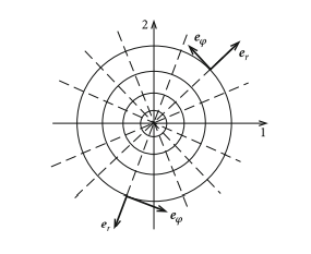
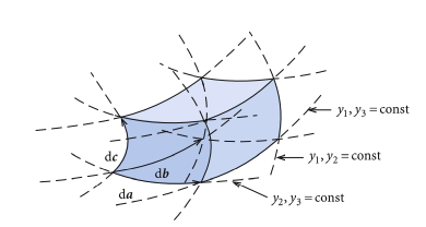
Before we inspect these relations using simple examples we want to formulate the characteristic parameters of a mass point $\mathbf{r}(t), \mathbf{v}(t), \mathbf{a}(t)$ in different systems of coordinates.
物理代写|理论力学作业代写Theoretical Mechanics代考|Simple Examples
(a) Mass Point on a Straight Line
We can describe the motion without referring to any special system of coordinates. If $\mathbf{c}$ is a vector in the direction of the motion and $\mathbf{b}$ a vector perpendicular to it then we can write for the position vector of the mass point (Fig. 2.4):
$$
\mathbf{r}(t)=\mathbf{b}+\alpha(t) \mathbf{c}
$$
From this, the respective time derivatives give us the velocity and acceleration:
$$
\mathbf{v}(t)=\dot{\alpha}(t) \mathbf{c} ; \quad \mathbf{a}(t)=\ddot{\alpha}(t) \mathbf{c}
$$
(b) Uniform Straight-Line Motion
Therewith it is meant the most simple form of motion, namely the one without any acceleration:
$$
\mathbf{a}(t)=0 ; \quad \mathbf{v}(t)=\mathbf{v}_{0} \quad \text { for all } t
$$
The third summand in $(2.2)$ then disappears:
$$
\mathbf{r}(t)=\mathbf{r}\left(t_{0}\right)+\mathbf{v}{0}\left(t-t{0}\right) .
$$
This formally agrees with (2.26). The motion is thus carried out rectilinearly in the direction of the constant velocity vector $\mathbf{v}{0}$. It is called ‘uniform’ since the same distances are covered in equal time intervals (Fig. 2.5). (c) Uniformly Accelerated Motion Now we assume a constant acceleration $$ \mathbf{a}(t)=\mathbf{a}{0}
$$
That means in (2.2):
$$
\begin{aligned}
\int_{t_{0}}^{t}\left[\int_{t_{0}}^{t^{\prime}} d t^{\prime \prime} \mathbf{a}\left(t^{\prime \prime}\right)\right] d t^{\prime} &=\int_{t_{0}}^{t}\left[\mathbf{a}{0}\left(t^{\prime}-t{0}\right)\right] d t^{\prime}=\
&=\mathbf{a}{0}\left(\frac{t^{2}}{2}-\frac{t{0}^{2}}{2}\right)-\mathbf{a}{0} t{0}\left(t-t_{0}\right)=\
&=\frac{1}{2} \mathbf{a}{0}\left(t-t{0}\right)^{2} .
\end{aligned}
$$
We therewith get as path line:
$$
\mathbf{r}(t)=\mathbf{r}\left(t_{0}\right)+\mathbf{v}\left(t_{0}\right)\left(t-t_{0}\right)+\frac{1}{2} \mathbf{a}{0}\left(t-t{0}\right)^{2} .
$$
The velocity of the mass point increases linearly with time (Fig. 2.6):
$$
\mathbf{v}(t)=\mathbf{v}\left(t_{0}\right)+\mathbf{a}{0}\left(t-t{0}\right)
$$
物理代写|理论力学作业代写Theoretical Mechanics代考|Fundamental Laws of Dynamics
Up to now we have restricted ourselves to describe the motion of a mass point without investigating the primary cause of the motion. From now on, the latter will be the focus of our considerations. The goal is to develop procedures by which one can derive the explicit movement of the mass point from a known driving cause.
We start with a few very general remarks concerning the challenges and possibilities of every physical theory; here, however, with the special perspective on Classical Mechanics. Like any physical theory mechanics also is based on
definitions and theorems
The definitions are reasonably separated into basis definitions and following definitions:
By basis definitions we mean concepts like position, time, mass, …, which are no further commented on in the course of the theory. Following definitions are entities derived from the basis definitions such as velocity, acceleration, momentum, … Analogously we have also to dccompose the theorenīs:
Axioms are a matter of basic empirical facts which are mathematically not provable and will not be further justified within the theory. In the framework of Classical Mechanics these are ‘Newton’s axloms of motion’. By concluslons we understand the actual results of the physical theory. By use of the concept of the “mathematical proof’ they emerge out of the basis definitions and axioms which together are called the postulates of the theory.
The ‘ultimate judge’ of any physical theory is the experiment. The value of a theory is measured by the degree of agreement of its conclusions with the manifestations of nature. It is known today that Classical Mechanics is not able to correctly describe all movements and manifestations of the inanimate nature. In particular in atomic and subatomic regions modifications have become necessary. But one can regard Classical Mechanics as a self-consistent limiting case of a higher all-embracing theory, if it is finally found.
理论力学代写
物理代写|理论力学作业代写Theoretical Mechanics代考|Velocity and Acceleration
质点运动的特点是:
位置向量:r(吨),
速度矢量:在(吨)=r˙(吨).
加速度矢量:一种(吨)=r¨(吨).
更高的时间导数使我们对力学不感兴趣。很多时候,它们甚至不存在,因为在许多实际情况下,加速度不是时间的连续函数。
力学的典型任务包括计算路径线(轨迹)r(吨)基于给定的加速度一种(吨)=r¨(吨). 为此,显然必须整合一种(吨)时间上的两倍。每次积分后,都会出现一个积分常数,除非我们有两个初始条件可供我们使用来固定这些常数,否则该积分常数仍未确定。在这方面,让我们假设我们知道质点(粒子)在某个时间的速度和位置吨0, IE
一种(吨) 对全部 吨,在(吨0), 和 r(吨0)
给出。那么粒子的速度由下式确定
在(吨)=在(吨0)+∫吨0吨d吨′一种(吨′)
和位置向量:
r(吨)=r(吨0)+在(吨0)(吨−吨0)+∫吨0吨[∫吨0吨′d吨′′一种(吨′′)]d吨′
在我们使用简单的例子检查这些关系之前,我们想制定一个质点的特征参数r(吨),在(吨),一种(吨)在不同的坐标系中。
物理代写|理论力学作业代写Theoretical Mechanics代考|Simple Examples
(a) 直线上
的质点 我们可以在不参考任何特殊坐标系的情况下描述运动。如果C是运动方向上的向量,并且b一个垂直于它的向量,那么我们可以写出质点的位置向量(图 2.4):
r(吨)=b+一种(吨)C
由此,各自的时间导数为我们提供了速度和加速度:
在(吨)=一种˙(吨)C;一种(吨)=一种¨(吨)C
(b) 匀速直线运动
它是指最简单的运动形式,即没有任何加速度的运动:
一种(吨)=0;在(吨)=在0 对全部 吨
第三条总括(2.2)然后消失:
r(吨)=r(吨0)+在0(吨−吨0).
这正式与(2.26)一致。运动因此在恒定速度矢量的方向上直线执行在0. 它被称为“均匀”,因为相同的距离以相同的时间间隔覆盖(图 2.5)。(c) 匀加速运动 现在我们假设一个匀加速
一种(吨)=一种0
这意味着在 (2.2) 中:
∫吨0吨[∫吨0吨′d吨′′一种(吨′′)]d吨′=∫吨0吨[一种0(吨′−吨0)]d吨′= =一种0(吨22−吨022)−一种0吨0(吨−吨0)= =12一种0(吨−吨0)2.
我们由此得到作为路径线:
r(吨)=r(吨0)+在(吨0)(吨−吨0)+12一种0(吨−吨0)2.
质点的速度随时间线性增加(图 2.6):
在(吨)=在(吨0)+一种0(吨−吨0)
物理代写|理论力学作业代写Theoretical Mechanics代考|Fundamental Laws of Dynamics
到目前为止,我们仅限于描述质点的运动,而没有研究运动的主要原因。从现在开始,后者将是我们考虑的重点。目标是开发程序,通过该程序可以从已知的驱动原因推导出质点的显式运动。
我们从关于每一个物理理论的挑战和可能性的一些非常笼统的评论开始;然而,在这里,以对经典力学的特殊视角。像任何物理理论一样,力学也是基于
定义和定理
的定义被合理地分为基础定义和以下定义:
我们所说的基础定义是指位置、时间、质量等概念,在理论过程中没有进一步评论。以下定义是从速度、加速度、动量等基本定义派生而来的实体……类似地,我们还必须对理论进行分解:
公理是基本经验事实的问题,在数学上无法证明,也不会在理论中进一步证明。在经典力学的框架中,这些是“牛顿运动轴”。通过结论,我们了解物理理论的实际结果。通过使用“数学证明”的概念,它们从基础定义和公理中出现,这些基础定义和公理一起被称为理论的假设。
任何物理理论的“终极裁判”都是实验。一个理论的价值是通过其结论与自然现象的一致程度来衡量的。今天众所周知,古典力学无法正确描述无生命自然的所有运动和表现。特别是在原子和亚原子区域的修改已成为必要。但是,如果最终找到经典力学,则可以将其视为更高的无所不包理论的自洽极限情况。

统计代写请认准statistics-lab™. statistics-lab™为您的留学生涯保驾护航。
金融工程代写
金融工程是使用数学技术来解决金融问题。金融工程使用计算机科学、统计学、经济学和应用数学领域的工具和知识来解决当前的金融问题,以及设计新的和创新的金融产品。
非参数统计代写
非参数统计指的是一种统计方法,其中不假设数据来自于由少数参数决定的规定模型;这种模型的例子包括正态分布模型和线性回归模型。
广义线性模型代考
广义线性模型(GLM)归属统计学领域,是一种应用灵活的线性回归模型。该模型允许因变量的偏差分布有除了正态分布之外的其它分布。
术语 广义线性模型(GLM)通常是指给定连续和/或分类预测因素的连续响应变量的常规线性回归模型。它包括多元线性回归,以及方差分析和方差分析(仅含固定效应)。
有限元方法代写
有限元方法(FEM)是一种流行的方法,用于数值解决工程和数学建模中出现的微分方程。典型的问题领域包括结构分析、传热、流体流动、质量运输和电磁势等传统领域。
有限元是一种通用的数值方法,用于解决两个或三个空间变量的偏微分方程(即一些边界值问题)。为了解决一个问题,有限元将一个大系统细分为更小、更简单的部分,称为有限元。这是通过在空间维度上的特定空间离散化来实现的,它是通过构建对象的网格来实现的:用于求解的数值域,它有有限数量的点。边界值问题的有限元方法表述最终导致一个代数方程组。该方法在域上对未知函数进行逼近。[1] 然后将模拟这些有限元的简单方程组合成一个更大的方程系统,以模拟整个问题。然后,有限元通过变化微积分使相关的误差函数最小化来逼近一个解决方案。
tatistics-lab作为专业的留学生服务机构,多年来已为美国、英国、加拿大、澳洲等留学热门地的学生提供专业的学术服务,包括但不限于Essay代写,Assignment代写,Dissertation代写,Report代写,小组作业代写,Proposal代写,Paper代写,Presentation代写,计算机作业代写,论文修改和润色,网课代做,exam代考等等。写作范围涵盖高中,本科,研究生等海外留学全阶段,辐射金融,经济学,会计学,审计学,管理学等全球99%专业科目。写作团队既有专业英语母语作者,也有海外名校硕博留学生,每位写作老师都拥有过硬的语言能力,专业的学科背景和学术写作经验。我们承诺100%原创,100%专业,100%准时,100%满意。
随机分析代写
随机微积分是数学的一个分支,对随机过程进行操作。它允许为随机过程的积分定义一个关于随机过程的一致的积分理论。这个领域是由日本数学家伊藤清在第二次世界大战期间创建并开始的。
时间序列分析代写
随机过程,是依赖于参数的一组随机变量的全体,参数通常是时间。 随机变量是随机现象的数量表现,其时间序列是一组按照时间发生先后顺序进行排列的数据点序列。通常一组时间序列的时间间隔为一恒定值(如1秒,5分钟,12小时,7天,1年),因此时间序列可以作为离散时间数据进行分析处理。研究时间序列数据的意义在于现实中,往往需要研究某个事物其随时间发展变化的规律。这就需要通过研究该事物过去发展的历史记录,以得到其自身发展的规律。
回归分析代写
多元回归分析渐进(Multiple Regression Analysis Asymptotics)属于计量经济学领域,主要是一种数学上的统计分析方法,可以分析复杂情况下各影响因素的数学关系,在自然科学、社会和经济学等多个领域内应用广泛。
MATLAB代写
MATLAB 是一种用于技术计算的高性能语言。它将计算、可视化和编程集成在一个易于使用的环境中,其中问题和解决方案以熟悉的数学符号表示。典型用途包括:数学和计算算法开发建模、仿真和原型制作数据分析、探索和可视化科学和工程图形应用程序开发,包括图形用户界面构建MATLAB 是一个交互式系统,其基本数据元素是一个不需要维度的数组。这使您可以解决许多技术计算问题,尤其是那些具有矩阵和向量公式的问题,而只需用 C 或 Fortran 等标量非交互式语言编写程序所需的时间的一小部分。MATLAB 名称代表矩阵实验室。MATLAB 最初的编写目的是提供对由 LINPACK 和 EISPACK 项目开发的矩阵软件的轻松访问,这两个项目共同代表了矩阵计算软件的最新技术。MATLAB 经过多年的发展,得到了许多用户的投入。在大学环境中,它是数学、工程和科学入门和高级课程的标准教学工具。在工业领域,MATLAB 是高效研究、开发和分析的首选工具。MATLAB 具有一系列称为工具箱的特定于应用程序的解决方案。对于大多数 MATLAB 用户来说非常重要,工具箱允许您学习和应用专业技术。工具箱是 MATLAB 函数(M 文件)的综合集合,可扩展 MATLAB 环境以解决特定类别的问题。可用工具箱的领域包括信号处理、控制系统、神经网络、模糊逻辑、小波、仿真等。