如果你也在 怎样代写电动力学electrodynamics这个学科遇到相关的难题,请随时右上角联系我们的24/7代写客服。
电动力学是物理学的一个分支,处理快速变化的电场和磁场。
statistics-lab™ 为您的留学生涯保驾护航 在代写电动力学electrodynamics方面已经树立了自己的口碑, 保证靠谱, 高质且原创的统计Statistics代写服务。我们的专家在代写电动力学electrodynamics代写方面经验极为丰富,各种代写电动力学electrodynamics相关的作业也就用不着说。
我们提供的电动力学electrodynamics及其相关学科的代写,服务范围广, 其中包括但不限于:
- Statistical Inference 统计推断
- Statistical Computing 统计计算
- Advanced Probability Theory 高等概率论
- Advanced Mathematical Statistics 高等数理统计学
- (Generalized) Linear Models 广义线性模型
- Statistical Machine Learning 统计机器学习
- Longitudinal Data Analysis 纵向数据分析
- Foundations of Data Science 数据科学基础
物理代写|电动力学代写electromagnetism代考|A Basic Stochastic Integral
The following is similar to Example $2 .$
Example 5 Suppose $s=1,2,3, \ldots$ is time, measured in days. Suppose a share, or unit of stock, has value $x(s)$ on day s; suppose $z(s)$ is the number of shares held on day $s$; and suppose $c(s)$ is the change in the value of the shareholding on day $s$ as a result of the change in share value from the previous day so $c(s)=$ $z(s-1)(x(s)-x(s-1))$. Let $w(s)$ be the cumulative change in shareholding value at end of day $s$, so $w(s)=w(s-1)+c(s)$. If share value $x(s)$ and stockholding $z(s)$ are subject to random variability, how is the gain (or loss) from the stockholding to be estimated?
Take initial value (at time $s=0)$ of the share to be $x(0)$ (or $\left.x_{0}\right)$, take the initial shareholding or number of shares owned to be $z(0)$ (or $\left.z_{0}\right)$. Then, at end of day $1(s=1)$,
$$
c(1)=z(0) \times(x(1)-x(0)), \quad w(1)=w(0)+c(1)=c(1)
$$
At end of day $s$,
$$
c(s)=z(s-1) \times(x(s)-x(s-1)), \quad w(s)=w(s-1)+c(s)
$$
After $t$ days,
$$
w(t)=\sum_{s=1}^{t} z(s-1)(x(s)-x(s-1)) .
$$
If the time increments are reduced to arbitrarily small size (so $s$ represents number of “time ticks” -fractions of a second, say), with the meaning of the other variables adjusted accordingly, then
$$
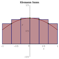
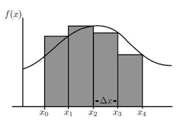
w(t)=\sum_{j=1}^{n} z\left(s_{j-1}\right)\left(x\left(s_{j}\right)-x\left(s_{j-1}\right)\right), \quad \text { or } \quad w(t)=\sum z(s) \Delta x(s)
$$
The latter expressions are Riemann sum estimates of $\int_{0}^{t} z(s) d x(s)$ (a Stieltjestype integral) whenever the latter exists.
Each of the expressions in (2.4) is sample value of a random variable
$$
W(t)=\sum_{j=1}^{n} Z\left(s_{j-1}\right)\left(X\left(s_{j}\right)-X\left(s_{j-1}\right)\right) \text { or } \int_{0}^{t} Z(s) d X(s)
$$constructed from the random variables $X, Z$, and $W$. These notations symbolize in a “naive” or “realistic” way-the stochastic integral of the process $Z$ with respect to the process $X$. In chapter 8 of [MTRV], symbols s, or $\mathbf{S}$, or $\mathcal{S}$ are used (in place of the symbol $\int$ ) for various kinds of stochastic integral. In the context described here, S would be the appropriate notation. (See (5.28) below.)
物理代写|电动力学代写electromagnetism代考|Choosing a Sample Space
It was mentioned earlier that there are many alternative ways of producing a sample space $\Omega$ (along with the linked probability measure $P$ and family $\mathcal{A}$ of measurable subsets of $\Omega$ ). The set of numbers
$$
{-5,-4,-3,-2,-1,0,1,2,3,4,5,10}
$$
was used as sample space for the random variability in the preceding example of stochastic integration. The measurable space $\mathcal{A}$ was the family of all subsets of $\Omega$, and the example was illustrated by means of two distinct probability measures $P$, one of which was based on Up and Down transitions being equally likely, where for the other measure an Up transition was twice as likely as a Down.
An alternative sample space for this example of random variability is
$$
\Omega=\Omega \Omega_{1} \times \Omega \Omega_{2} \times \Omega \Omega_{3} \times \Omega \Omega_{4}
$$
where $\Omega_{j}={U, D}$ for $j=1,2,3,4$; so the elements $\omega$ of $\Omega$ consist of sixteen 4-tuples of the form
$$
\omega=(\cdot, \cdot \cdot \cdot), \quad \text { such as } \omega=(U, D, D, U) \text { for example. }
$$
Let the measurable space $\mathcal{A}$ be the family of all subsets $A$ of $\Omega$; so $\mathcal{A}$ contains $2^{16}$ members, one of which (for example) is
$$
A={(D, U, U, D),(U, D, D, U),(D, U, D, U),(U, U, U, U),(D, D, D, D)}
$$
with $A$ consisting of five individual four-tuples. Assume that Up transitions and Down transitions are equally likely, and that they are independent events. Then, as before,
$$
P({\omega})=\frac{1}{16}
$$
for each $\omega \in \Omega$. For $A$ above, $P(A)=\frac{5}{16}$.
To relate this probability structure to the shareholding example, let $\mathbf{R}^{4}=$ $\mathbf{R} \times \mathbf{R} \times \mathbf{R} \times \mathbf{R}$, and let
$$
f: \Omega \mapsto \mathbf{R}^{4}, \quad f(\omega)=((x(1), x(2), x(3), x(4)),
$$
using Table 2.4; so, for instance,
$$
f(\omega)=f((U, D, D, U))=(11,10,9,10)=(x(1), x(2), x(3), x(4)),
$$
and so on. Next, let $\mathbf{S}$ denote the stochastic integrals of the preceding section, so for $x=(x(1), x(2), x(3), x(4)) \in \mathbf{R}^{4}$,
$$
\mathbf{S}(x)=\int_{0}^{4} z(s) d x(s)=\sum_{s=1}^{4} z(s-1)(x(s)-x(s-1)),
$$
so $\mathbf{S}(x)$ gives the values $w(4)$ of Table 2.4. As described in Section $2.3$, the rationale for deducing the probabilities of outcomes $\mathbf{S}(x)$, = $w(4)$, from the probabilities on $\Omega$ is the relationship
$$
P(w(4))=P\left(f^{-1}\left(\mathbf{S}^{-1}(w(4))\right)\right) .
$$
物理代写|电动力学代写electromagnetism代考|More on Basic Stochastic Integral
The constructions in Sections $2.3$ and $2.4$ purported to be about stochastic integration. While a case can be made that (2.6) and (2.7) are actually stochastic integrals, such simple examples are not really what the standard or classical theory of Chapter 1 is all about. The examples and illustrations in Sections $2.3$ and $2.4$ may not really be much help in coming to grips with the standard theory of stochastic integrals outlined in Chapter $1 .$
This is because Chapter 1, on the definition and meaning of classical stochastic integration, involves subtle passages to a limit, whereas (2.6) and (2.7) involve only finite sums and some elementary probability calculations.
From the latter point of view, introducing probability measure spaces and random-variables-as-measurable-functions seems to be an unnecessary complication. So, from such a straightforward starting point, why does the theory become so challenging and “messy”, as portrayed in Chapter $1 ?$
As in Example 2, the illustration in Section $2.3$ involves dividing up the time period (4 days) into 4 sections; leading to sample space $\Omega=\mathbf{R}^{4}$ in (2.15). Why not simply continue in this vein, and subdivide the time into 40 , or 400 , or 4 million steps instead of just 4 ; using sample spaces $\mathbf{R}^{40}$, or $\mathbf{R}^{400}$, or $\mathbf{R}^{4000000}$, respectively? The computations may become lengthier, but no new principle is involved; each of the variables changes in discrete steps at discrete points in time. ${ }^{5}$
Other simplifications can be similarly adopted. For instance, only two kinds of changes are contemplated in Section 2.3: increase (Up) or decrease (Down).
电动力学代考
物理代写|电动力学代写electromagnetism代考|A Basic Stochastic Integral
以下与示例类似2.
示例 5 假设s=1,2,3,…是时间,以天为单位。假设股票或股票单位具有价值X(s)在第 s 天;认为和(s)是当天持有的股票数量s; 并假设C(s)是当天股权价值的变化s由于前一天股票价值的变化,所以C(s)= 和(s−1)(X(s)−X(s−1)). 让在(s)是日终股权价值的累积变化s, 所以在(s)=在(s−1)+C(s). 如果股票价值X(s)和持股和(s)受随机变量的影响,如何估计持股的收益(或损失)?
取初始值(在时间s=0)的份额是X(0)(或者X0), 取初始持股量或拥有的股份数量为和(0)(或者和0). 然后,在一天结束时1(s=1),
C(1)=和(0)×(X(1)−X(0)),在(1)=在(0)+C(1)=C(1)
在一天结束时s,
C(s)=和(s−1)×(X(s)−X(s−1)),在(s)=在(s−1)+C(s)
后吨天,
在(吨)=∑s=1吨和(s−1)(X(s)−X(s−1)).
如果时间增量减少到任意小的大小(所以s表示“时间滴答”的数量 – 秒的分数,例如),其他变量的含义相应调整,然后
在(吨)=∑j=1n和(sj−1)(X(sj)−X(sj−1)), 或者 在(吨)=∑和(s)ΔX(s)
后面的表达式是黎曼和估计∫0吨和(s)dX(s)(一个 Stieltjestype 积分)只要后者存在。
(2.4)中的每个表达式都是随机变量的样本值
在(吨)=∑j=1n从(sj−1)(X(sj)−X(sj−1)) 或者 ∫0吨从(s)dX(s)由随机变量构成X,从, 和在. 这些符号以“朴素”或“现实”的方式象征着过程的随机积分从关于过程X. 在 [MTRV] 的第 8 章中,符号 s 或小号, 或者小号被使用(代替符号∫) 用于各种随机积分。在此处描述的上下文中,S 将是适当的符号。(见下文(5.28)。)
物理代写|电动力学代写electromagnetism代考|Choosing a Sample Space
前面提到过,产生样本空间的方法有很多Ω(连同关联的概率测度磷和家人一个的可测量子集Ω)。数字集
−5,−4,−3,−2,−1,0,1,2,3,4,5,10
在前面的随机积分示例中,它被用作随机变异性的样本空间。可测空间一个是所有子集的族Ω, 这个例子是通过两个不同的概率测度来说明的磷,其中一个基于向上和向下转换的可能性相同,而对于另一种度量,向上转换的可能性是向下转换的两倍。
这个随机变异性示例的替代样本空间是
Ω=ΩΩ1×ΩΩ2×ΩΩ3×ΩΩ4
在哪里Ωj=在,D为了j=1,2,3,4; 所以元素ω的Ω由 16 个 4 元组组成
ω=(⋅,⋅⋅⋅), 如 ω=(在,D,D,在) 例如。
让可测量的空间一个是所有子集的族一个的Ω; 所以一个包含216成员,其中之一(例如)是
一个=(D,在,在,D),(在,D,D,在),(D,在,D,在),(在,在,在,在),(D,D,D,D)
和一个由五个单独的四元组组成。假设向上转换和向下转换的可能性相同,并且它们是独立事件。然后,和以前一样,
磷(ω)=116
对于每个ω∈Ω. 为了一个以上,磷(一个)=516.
为了将此概率结构与股权示例联系起来,让R4= R×R×R×R, 然后让
F:Ω↦R4,F(ω)=((X(1),X(2),X(3),X(4)),
使用表 2.4;所以,例如,
F(ω)=F((在,D,D,在))=(11,10,9,10)=(X(1),X(2),X(3),X(4)),
等等。接下来,让小号表示上一节的随机积分,所以对于X=(X(1),X(2),X(3),X(4))∈R4,
小号(X)=∫04和(s)dX(s)=∑s=14和(s−1)(X(s)−X(s−1)),
所以小号(X)给出值在(4)表 2.4。如部分所述2.3,推断结果概率的基本原理小号(X), = 在(4),从概率上Ω是关系
磷(在(4))=磷(F−1(小号−1(在(4)))).
物理代写|电动力学代写electromagnetism代考|More on Basic Stochastic Integral
部分中的结构2.3和2.4据称是关于随机积分。虽然可以证明 (2.6) 和 (2.7) 实际上是随机积分,但这些简单的例子并不是第 1 章的标准或经典理论的全部内容。章节中的示例和插图2.3和2.4可能对掌握第 1 章中概述的标准随机积分理论没有太大帮助1.
这是因为第 1 章,关于经典随机积分的定义和含义,涉及到一个极限的微妙通道,而(2.6)和(2.7)只涉及有限和和一些基本的概率计算。
从后者的角度来看,引入概率测度空间和随机变量作为可测量函数似乎是不必要的复杂化。那么,从这样一个直截了当的出发点,为什么这个理论会变得如此具有挑战性和“混乱”,正如本章所描述的那样1?
与示例 2 一样,第 2 节中的插图2.3涉及将时间段(4天)分成4个部分;导致样本空间Ω=R4在(2.15)中。为什么不简单地继续这种方式,将时间细分为 40 或 400 或 400 万步,而不仅仅是 4 ;使用样本空间R40, 或者R400, 或者R4000000, 分别?计算可能会变长,但没有涉及新的原理;每个变量在离散的时间点以离散的步骤变化。5
可以类似地采用其他简化。例如,在第 2.3 节中只考虑了两种变化:增加(Up)或减少(Down)。

统计代写请认准statistics-lab™. statistics-lab™为您的留学生涯保驾护航。
金融工程代写
金融工程是使用数学技术来解决金融问题。金融工程使用计算机科学、统计学、经济学和应用数学领域的工具和知识来解决当前的金融问题,以及设计新的和创新的金融产品。
非参数统计代写
非参数统计指的是一种统计方法,其中不假设数据来自于由少数参数决定的规定模型;这种模型的例子包括正态分布模型和线性回归模型。
广义线性模型代考
广义线性模型(GLM)归属统计学领域,是一种应用灵活的线性回归模型。该模型允许因变量的偏差分布有除了正态分布之外的其它分布。
术语 广义线性模型(GLM)通常是指给定连续和/或分类预测因素的连续响应变量的常规线性回归模型。它包括多元线性回归,以及方差分析和方差分析(仅含固定效应)。
有限元方法代写
有限元方法(FEM)是一种流行的方法,用于数值解决工程和数学建模中出现的微分方程。典型的问题领域包括结构分析、传热、流体流动、质量运输和电磁势等传统领域。
有限元是一种通用的数值方法,用于解决两个或三个空间变量的偏微分方程(即一些边界值问题)。为了解决一个问题,有限元将一个大系统细分为更小、更简单的部分,称为有限元。这是通过在空间维度上的特定空间离散化来实现的,它是通过构建对象的网格来实现的:用于求解的数值域,它有有限数量的点。边界值问题的有限元方法表述最终导致一个代数方程组。该方法在域上对未知函数进行逼近。[1] 然后将模拟这些有限元的简单方程组合成一个更大的方程系统,以模拟整个问题。然后,有限元通过变化微积分使相关的误差函数最小化来逼近一个解决方案。
tatistics-lab作为专业的留学生服务机构,多年来已为美国、英国、加拿大、澳洲等留学热门地的学生提供专业的学术服务,包括但不限于Essay代写,Assignment代写,Dissertation代写,Report代写,小组作业代写,Proposal代写,Paper代写,Presentation代写,计算机作业代写,论文修改和润色,网课代做,exam代考等等。写作范围涵盖高中,本科,研究生等海外留学全阶段,辐射金融,经济学,会计学,审计学,管理学等全球99%专业科目。写作团队既有专业英语母语作者,也有海外名校硕博留学生,每位写作老师都拥有过硬的语言能力,专业的学科背景和学术写作经验。我们承诺100%原创,100%专业,100%准时,100%满意。
随机分析代写
随机微积分是数学的一个分支,对随机过程进行操作。它允许为随机过程的积分定义一个关于随机过程的一致的积分理论。这个领域是由日本数学家伊藤清在第二次世界大战期间创建并开始的。
时间序列分析代写
随机过程,是依赖于参数的一组随机变量的全体,参数通常是时间。 随机变量是随机现象的数量表现,其时间序列是一组按照时间发生先后顺序进行排列的数据点序列。通常一组时间序列的时间间隔为一恒定值(如1秒,5分钟,12小时,7天,1年),因此时间序列可以作为离散时间数据进行分析处理。研究时间序列数据的意义在于现实中,往往需要研究某个事物其随时间发展变化的规律。这就需要通过研究该事物过去发展的历史记录,以得到其自身发展的规律。
回归分析代写
多元回归分析渐进(Multiple Regression Analysis Asymptotics)属于计量经济学领域,主要是一种数学上的统计分析方法,可以分析复杂情况下各影响因素的数学关系,在自然科学、社会和经济学等多个领域内应用广泛。
MATLAB代写
MATLAB 是一种用于技术计算的高性能语言。它将计算、可视化和编程集成在一个易于使用的环境中,其中问题和解决方案以熟悉的数学符号表示。典型用途包括:数学和计算算法开发建模、仿真和原型制作数据分析、探索和可视化科学和工程图形应用程序开发,包括图形用户界面构建MATLAB 是一个交互式系统,其基本数据元素是一个不需要维度的数组。这使您可以解决许多技术计算问题,尤其是那些具有矩阵和向量公式的问题,而只需用 C 或 Fortran 等标量非交互式语言编写程序所需的时间的一小部分。MATLAB 名称代表矩阵实验室。MATLAB 最初的编写目的是提供对由 LINPACK 和 EISPACK 项目开发的矩阵软件的轻松访问,这两个项目共同代表了矩阵计算软件的最新技术。MATLAB 经过多年的发展,得到了许多用户的投入。在大学环境中,它是数学、工程和科学入门和高级课程的标准教学工具。在工业领域,MATLAB 是高效研究、开发和分析的首选工具。MATLAB 具有一系列称为工具箱的特定于应用程序的解决方案。对于大多数 MATLAB 用户来说非常重要,工具箱允许您学习和应用专业技术。工具箱是 MATLAB 函数(M 文件)的综合集合,可扩展 MATLAB 环境以解决特定类别的问题。可用工具箱的领域包括信号处理、控制系统、神经网络、模糊逻辑、小波、仿真等。