如果你也在 怎样代写计量经济学Econometrics这个学科遇到相关的难题,请随时右上角联系我们的24/7代写客服。
计量经济学,对经济关系的统计和数学分析,通常作为经济预测的基础。这些信息有时被政府用来制定经济政策,也被私人企业用来帮助价格、库存和生产方面的决策。
statistics-lab™ 为您的留学生涯保驾护航 在代写计量经济学Econometrics方面已经树立了自己的口碑, 保证靠谱, 高质且原创的统计Statistics代写服务。我们的专家在代写计量经济学Econometrics代写方面经验极为丰富,各种代写计量经济学Econometrics相关的作业也就用不着说。
我们提供的计量经济学Econometrics及其相关学科的代写,服务范围广, 其中包括但不限于:
- Statistical Inference 统计推断
- Statistical Computing 统计计算
- Advanced Probability Theory 高等概率论
- Advanced Mathematical Statistics 高等数理统计学
- (Generalized) Linear Models 广义线性模型
- Statistical Machine Learning 统计机器学习
- Longitudinal Data Analysis 纵向数据分析
- Foundations of Data Science 数据科学基础
经济代写|计量经济学作业代写Econometrics代考|The Distribution of Wages
Suppose that we are interested in wage rates in the United States. Since wage rates vary across workers, we cannot describe wage rates by a single number. Instead, we can describe wages using a probability distribution. Formally, we view the wage of an individual worker as a random variable wage with the probability distribution
$$
F(u)=\mathbb{P}[w a g e \leq u]
$$
When we say that a person’s wage is random we mean that we do not know their wage before it is measured, and we treat observed wage rates as realizations from the distribution $F$. Treating unobserved wages as random variables and observed wages as realizations is a powerful mathematical abstraction which allows us to use the tools of mathematical probability.
A useful thought experiment is to imagine dialing a telephone number selected at random, and then asking the person who responds tn tell ws their wage rate. (Assıme for simplicity that all workers have. equal access to telephones, and that the person who answers your call will respond honestly.) In this thought experiment, the wage of the person you have called is a single draw from the distribution $F$ of wages in the population. By making many such phone calls we can learn the distribution $F$ of the entire population.
When a distribution function $F$ is differentiable we define the probability density function
$$
f(u)=\frac{d}{d u} F(u) .
$$
The density contains the same information as the distribution function, but the density is typically easier to visually interpret.
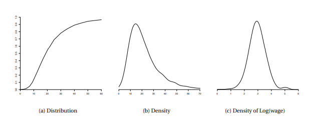
In Figure $2.1$ we display estimates ${ }^{1}$ of the probability distribution function (panel (a)) and density function (panel (b)) of U.S. wage rates in 2009 . We see that the density is peaked around $\$ 15$, and most of the probability mass appears to lie between $\$ 10$ and $\$ 40$. These are ranges for typical wage rates in the U.S. population.
Important measures of central tendency are the median and the mean. The median $m$ of a continuous ${ }^{2}$ distribution $F$ is the unique solution to
$$
F(m)=\frac{1}{2}
$$
The median U.S. wage is $\$ 19.23$. The median is a robust ${ }^{3}$ measure of central tendency, but it is tricky to use for many calculations as it is not a linear operator.
The expectation or mean of a random variable $y$ with discrete support is
$$
\mu=\mathbb{E}[y]=\sum_{j=1}^{\infty} \tau_{j} \mathbb{P}\left[y=\tau_{j}\right]
$$
For a continuous random variable with density $f(y)$ the expectation is
$$
\mu=\mathbb{E}[y]=\int_{-\infty}^{\infty} y f(y) d y .
$$
Here we have used the common and convenient convention of using the single character $y$ to denote a random variable, rather than the more cumbersome label wage. We sometimes use the notation Ey instead of $E[y]$ when the variable whose expectation is being taken is clear from the context. There is no distinction in meaning. An alternative notation which includes both discrete and continuous random variables as special cases is
$$
\mu=\mathbb{E}[y]=\int_{-\infty}^{\infty} y d F(y)
$$
经济代写|计量经济学作业代写Econometrics代考|Conditional Expectation
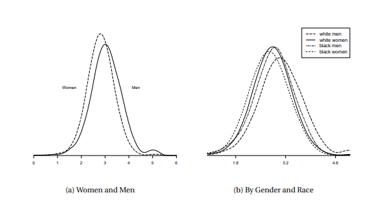
We saw in Figure ?? the density of log wages. Is this distribution the same for all workers, or does the wage distribution vary across subpopulations? To answer this question, we can compare wage distributions for different groups – for example, men and women. The plot on the left in Figure $2.2$ displays the densities of log wages for U.S. men and women. We can see that the two wage densities take similar shapes but the density for men is somewhat shifted to the right.
The values $3.05$ and $2.81$ are the mean log wages in the subpopulations of men and women workers. They are called the conditional means (or conditional expectations) of log wages given gender. We can write their specific values as
$$
\begin{gathered}
\mathbb{E}[\log (\text { wage }) \mid \text { gender }=\text { man }]=3.05 \
\mathbb{E}[\log (\text { wage }) \mid \text { gender }=\text { woman }]=2.81 .
\end{gathered}
$$
We call these means conditional as they are conditioning on a fixed value of the variable gender. While you might not think of a person’s gender as a random variable, it is random from the viewpoint of econometric analysis. If you randomly select an individual, the gender of the individual is unknown and thus random. (In the population of U.S. workers, the probability that a worker is a woman happens to be 43\%.) In observational data, it is most appropriate to view all measurements as random variables, and the means of subpopulatlons are then conditlonal means.
As the two densities in Figure $2.2$ appear similar, a hasty inference might be that there is not a meaningful difference between the wage distributions of men and women. Before jumping to this conclusion let us examine the differences in the distributions more carefully. As we mentioned above, the primary difference between the two densities appears to be their means. This difference equals
$$
\begin{aligned}
\mathbb{E}[\log (\text { wage }) \mid \text { gender }=\text { man }]-\mathbb{E}[\log (\text { wage }) \mid \text { gender }=\text { woman }] &=3.05-2.81 \
&=0.24 .
\end{aligned}
$$
A difference in expected log wages of $0.24$ is often interpreted as an average $24 \%$ difference between the wages of men and women, which is quite substantial. (For a more complete explanation see Section 2.4.)
Consider further splitting the men and women subpopulations by race, dividing the population into whites, blacks, and other races. We display the log wage density functions of four of these groups on the right in Figure 2.2. Again we see that the primary difference between the four density functions is their central tendency.
Focusing on the means of these distributions, Table $2.1$ reports the mean log wage for each of the six sub-populations.
Table 2.1: Mean Log Wages by Gender and Race
\begin{tabular}{lcc}
\hline \hline & men & women \
\cline { 2 – 3 } white & $3.07$ & $2.82$ \
black & $2.86$ & $2.73$ \
other & $3.03$ & $2.86$ \
\hline
\end{tabular}
The entries in Table $2.1$ are the conditional means of $\log ($ wage $)$ given gender and race. For example
$$
\mathbb{E}[\log (\text { wage }) \mid \text { gender }=\text { man, race }=\text { white }]=3.07
$$
and
$$
\mathbb{E}[\log (\text { wage }) \mid \text { gender }=\text { woman }, \text { race }=\text { black }]=2.73
$$
经济代写|计量经济学作业代写Econometrics代考|Log Differences
A useful approximation for the natural logarithm for small $x$ is
$$
\log (1+x) \approx x
$$
This can be derived from the infinite series expansion of $\log (1+x)$ :
$$
\begin{aligned}
\log (1+x) &=x-\frac{x^{2}}{2}+\frac{x^{3}}{3}-\frac{x^{4}}{4}+\cdots \
&=x+O\left(x^{2}\right)
\end{aligned}
$$
The symbol $O\left(x^{2}\right)$ means that the remainder is bounded by $A x^{2}$ as $x \rightarrow 0$ for some $A<\infty$. Numerically, the approximation $\log (1+x) \simeq x$ is within $0.001$ for $|x| \leq 0.1$. The approximation error increases with $|x|$.
If $y^{}$ is $c \%$ greater than $y$ then $$ y^{}=(1+c / 100) y
$$
Taking natural logarithms,
$$
\log y^{}=\log y+\log (1+c / 100) $$ or $$ \log y^{}-\log y=\log (1+c / 100) \approx \frac{c}{100}
$$
where the approximation is (2.2). This shows that 100 multiplied by the difference in logarithms is approximately the percentage difference between $y$ and $y^{*}$. Numerically, the approximation error is less than $0.1$ percentage points for $|c| \leq 10$.
Many econometric equations take the semi-log form
$$
\begin{aligned}
&\mathbb{E}[\log (w) \mid \operatorname{group}=1]=a_{1} \
&\mathbb{E}[\log (w) \mid \operatorname{group}=2]=a_{2}
\end{aligned}
$$
How should we interpret the difference $\Delta=a_{1}-a_{2}$ ? In the previous section we stated that this difference is often interpreted as the average percentage difference. This is not quite right, but is not quite wrong either.
As mentioned earlier, the geometric mean of a random variable $w$ is $\theta=\exp (\mathbb{E}[\log (w)])$. Thus $\theta_{1}=\exp \left(a_{1}\right)$ and $\theta_{2}=\exp \left(a_{2}\right)$ are the conditional geometric means for group 1 and group 2 . The geometric mean is a measure of central tendency, different from the arithmetic mean, and often closer to the median. The difference $\Delta=\mu_{1}-\mu_{2}$ is the difference in the logarithms between the two geometric
means. Thus by the above discussion about log differences $\Delta$ approximately equals the percentage difference between the conditional geometric means $\theta_{1}$ and $\theta_{2}$. The approximation is good for percentage differences less than $10 \%$ and the approximation deteriorates for percentages above that.
To compare different measures of percentage difference in our example see Table 2.2. In the first two columns we report average wages for men and women in the CPS population using three “averages”: mean (arithmetic), median, and geometric mean. For both groups the mean is higher than the median and geometric mean, and the latter two are similar to one another. This is a common feature of skewed distributions such as the wage distribution. The next two columns report the percentage differences between the first two columns. There are two ways of computing a percentage difference depending on which is the baseline. The third column reports the percentage difference taking the average woman’s wage as the baseline, so for example the first entry of $34 \%$ states that the mean wage for men is $34 \%$ higher than the mean wage for women. The fourth column reports the percentage difference taking the average men’s wage as the baseline. For example the first entry of $-25 \%$ states that the mean wage for women is $25 \%$ less than the mean wage for men.
Table $2.2$ shows that when examining average wages the difference between women’s and men’s wages is $25-34 \%$ depending on the baseline. If we examine the median wage the difference is $20-26 \%$. If we examine the geometric mean we find a difference of $21-26 \%$. The percentage difference in mean wages is considerably different from the other two measures as they measure different features of the distribution.
Returning to the log difference in equation (2.1), we found that the difference in the mean logarithm between men and women is $0.24$, and we stated that this is often interpreted as implying a $24 \%$ average percentage difference. More accurately it should be described as the approximate percentage difference in the geometric mean. Indeed, we see that that the actual percentage difference in the geometric mean is $21-26 \%$, depending on the baseline, which is quite similar to the difference in the mean logarithm.
What this implies in practice is that when we transform our data by taking logarithms (as is common in economics) and then compare means (including regression coefficients) we are computing approximate percentage differences in the average as measured by the geometric mean.
计量经济学代写
经济代写|计量经济学作业代写Econometrics代考|The Distribution of Wages
假设我们对美国的工资率感兴趣。由于工人的工资率不同,我们不能用一个数字来描述工资率。相反,我们可以使用概率分布来描述工资。形式上,我们将单个工人的工资视为具有概率分布的随机变量工资
F(在)=磷[在一种G和≤在]
当我们说一个人的工资是随机的时,我们的意思是在测量之前我们不知道他们的工资,我们将观察到的工资率视为分布的实现F. 将未观察到的工资视为随机变量,将观察到的工资视为实现是一种强大的数学抽象,它允许我们使用数学概率工具。
一个有用的思想实验是想象拨打一个随机选择的电话号码,然后让接听电话的人告诉他们他们的工资率。(为简单起见,假设所有工人都可以平等地使用电话,并且接听电话的人会诚实地回应。)在这个思想实验中,你所打电话的人的工资是从分配中抽取的一次F人口中的工资。通过拨打许多这样的电话,我们可以了解分布情况F全体人口的。
当分布函数F是可微的 我们定义概率密度函数
F(在)=dd在F(在).
密度包含与分布函数相同的信息,但密度通常更易于直观解释。
如图2.1我们显示估计12009年美国工资率的概率分布函数(图(a))和密度函数(图(b))。我们看到密度达到峰值$15,并且大部分概率质量似乎位于$10和$40. 这些是美国人口中典型工资率的范围。
集中趋势的重要度量是中位数和平均值。中位数米连续的2分配F是唯一的解决方案
F(米)=12
美国工资中位数是$19.23. 中位数是稳健的3集中趋势的度量,但由于它不是线性算子,因此在许多计算中使用起来很棘手。
随机变量的期望或均值是离散支持是
μ=和[是]=∑j=1∞τj磷[是=τj]
对于具有密度的连续随机变量F(是)期望是
μ=和[是]=∫−∞∞是F(是)d是.
在这里,我们使用了使用单个字符的常见且方便的约定是来表示一个随机变量,而不是更繁琐的标签工资。我们有时使用符号 Ey 而不是和[是]当从上下文中清楚地了解其期望的变量时。含义上没有区别。另一种包括离散和连续随机变量作为特殊情况的符号是
μ=和[是]=∫−∞∞是dF(是)
经济代写|计量经济学作业代写Econometrics代考|Conditional Expectation
我们在图中看到了?? 对数工资的密度。这种分布对所有工人来说都是一样的,还是工资分布在不同的子人群中有所不同?为了回答这个问题,我们可以比较不同群体的工资分布——例如,男性和女性。图左侧的情节2.2显示美国男性和女性的对数工资密度。我们可以看到这两种工资密度具有相似的形状,但男性的密度稍微向右移动。
价值3.05和2.81是男性和女性工人亚群的平均对数工资。它们被称为给定性别的对数工资的条件平均值(或条件期望)。我们可以将它们的具体值写为
和[日志( 工资 )∣ 性别 = 男人 ]=3.05 和[日志( 工资 )∣ 性别 = 女士 ]=2.81.
我们称这些方法为有条件的,因为它们以变量性别的固定值为条件。虽然您可能不会将一个人的性别视为随机变量,但从计量经济学分析的角度来看,它是随机的。如果你随机选择一个人,这个人的性别是未知的,因此是随机的。(在美国工人群体中,工人是女性的概率恰好是 43%。)在观察数据中,将所有测量值视为随机变量是最合适的,然后子群体的平均值就是条件平均值。
如图中的两个密度2.2看起来相似,草率的推论可能是男性和女性的工资分配之间没有有意义的差异。在得出这个结论之前,让我们更仔细地检查分布的差异。正如我们上面提到的,两种密度之间的主要区别似乎是它们的平均值。这个差等于
和[日志( 工资 )∣ 性别 = 男人 ]−和[日志( 工资 )∣ 性别 = 女士 ]=3.05−2.81 =0.24.
预期原木工资的差异0.24通常被解释为平均值24%男女工资差距,相当可观。(有关更完整的解释,请参见第 2.4 节。)
考虑进一步按种族划分男性和女性亚群,将人口分为白人、黑人和其他种族。我们在图 2.2 的右侧显示了其中四个组的对数工资密度函数。我们再次看到四个密度函数之间的主要区别在于它们的集中趋势。
着眼于这些分布的手段,表2.1报告六个子群体中每一个的平均对数工资。
表 2.1:按性别和种族划分的平均对数工资
\begin{tabular}{lcc} \hline \hline & men & women \ \cline { 2 – 3 } white & $3.07$ & $2.82$ \ black & $2.86$ & $2.73$ \ other & $3.03$ & $2.86$ \ \hline \end{表格}\begin{tabular}{lcc} \hline \hline & men & women \ \cline { 2 – 3 } white & $3.07$ & $2.82$ \ black & $2.86$ & $2.73$ \ other & $3.03$ & $2.86$ \ \hline \end{表格}
表中的条目2.1是有条件的手段日志(工资)考虑到性别和种族。例如
和[日志( 工资 )∣ 性别 = 人,种族 = 白色的 ]=3.07
和
和[日志( 工资 )∣ 性别 = 女士 , 种族 = 黑色的 ]=2.73
经济代写|计量经济学作业代写Econometrics代考|Log Differences
一个有用的近似自然对数的小X是
日志(1+X)≈X
这可以从无限级数展开推导出来日志(1+X) :
日志(1+X)=X−X22+X33−X44+⋯ =X+这(X2)
符号这(X2)表示余数有界一种X2作为X→0对于一些一种<∞. 在数值上,近似值日志(1+X)≃X是在0.001为了|X|≤0.1. 近似误差随着|X|.
如果是是C%比…更棒是然后是=(1+C/100)是
取自然对数,
日志是=日志是+日志(1+C/100)或者日志是−日志是=日志(1+C/100)≈C100
其中近似值为 (2.2)。这表明 100 乘以对数差异大约是两者之间的百分比差异是和是∗. 在数值上,近似误差小于0.1个百分点|C|≤10.
许多计量经济学方程采用半对数形式
和[日志(在)∣团体=1]=一种1 和[日志(在)∣团体=2]=一种2
我们应该如何解释差异Δ=一种1−一种2? 在上一节中,我们指出这种差异通常被解释为平均百分比差异。这并不完全正确,但也不是完全错误。
如前所述,随机变量的几何平均值在是θ=经验(和[日志(在)]). 因此θ1=经验(一种1)和θ2=经验(一种2)是组 1 和组 2 的条件几何平均值。几何平均值是集中趋势的度量,不同于算术平均值,并且通常更接近中位数。区别Δ=μ1−μ2是两个几何图形之间的对数差
方法。因此通过上面关于日志差异的讨论Δ大约等于条件几何平均值之间的百分比差异θ1和θ2. 该近似值适用于小于的百分比差异10%并且对于高于此的百分比,近似值会恶化。
要比较我们示例中不同的百分比差异度量,请参见表 2.2。在前两列中,我们使用三个“平均值”报告 CPS 人群中男性和女性的平均工资:平均值(算术)、中位数和几何平均值。两组的平均值都高于中位数和几何平均值,后两者相似。这是偏态分布(例如工资分布)的共同特征。接下来的两列报告前两列之间的百分比差异。有两种计算百分比差异的方法,具体取决于哪个是基线。第三列报告了以女性平均工资为基准的百分比差异,例如第一个条目34%指出男性的平均工资是34%高于女性的平均工资。第四列报告了以男性平均工资为基准的百分比差异。例如第一个条目−25%指出女性的平均工资是25%低于男性的平均工资。
桌子2.2表明在检查平均工资时,男女工资之间的差异为25−34%取决于基线。如果我们检查工资中位数,则差异为20−26%. 如果我们检查几何平均值,我们会发现差异为21−26%. 平均工资的百分比差异与其他两个衡量标准有很大不同,因为它们衡量的是分布的不同特征。
回到方程(2.1)中的对数差异,我们发现男性和女性之间的平均对数差异为0.24,我们说这通常被解释为暗示24%平均百分比差异。更准确地说,它应该被描述为几何平均值的近似百分比差异。事实上,我们看到几何平均值的实际百分比差异是21−26%,取决于基线,这与平均对数的差异非常相似。
这在实践中意味着,当我们通过取对数(在经济学中很常见)来转换我们的数据,然后比较平均值(包括回归系数)时,我们正在计算由几何平均值测量的平均值的近似百分比差异。

统计代写请认准statistics-lab™. statistics-lab™为您的留学生涯保驾护航。
金融工程代写
金融工程是使用数学技术来解决金融问题。金融工程使用计算机科学、统计学、经济学和应用数学领域的工具和知识来解决当前的金融问题,以及设计新的和创新的金融产品。
非参数统计代写
非参数统计指的是一种统计方法,其中不假设数据来自于由少数参数决定的规定模型;这种模型的例子包括正态分布模型和线性回归模型。
广义线性模型代考
广义线性模型(GLM)归属统计学领域,是一种应用灵活的线性回归模型。该模型允许因变量的偏差分布有除了正态分布之外的其它分布。
术语 广义线性模型(GLM)通常是指给定连续和/或分类预测因素的连续响应变量的常规线性回归模型。它包括多元线性回归,以及方差分析和方差分析(仅含固定效应)。
有限元方法代写
有限元方法(FEM)是一种流行的方法,用于数值解决工程和数学建模中出现的微分方程。典型的问题领域包括结构分析、传热、流体流动、质量运输和电磁势等传统领域。
有限元是一种通用的数值方法,用于解决两个或三个空间变量的偏微分方程(即一些边界值问题)。为了解决一个问题,有限元将一个大系统细分为更小、更简单的部分,称为有限元。这是通过在空间维度上的特定空间离散化来实现的,它是通过构建对象的网格来实现的:用于求解的数值域,它有有限数量的点。边界值问题的有限元方法表述最终导致一个代数方程组。该方法在域上对未知函数进行逼近。[1] 然后将模拟这些有限元的简单方程组合成一个更大的方程系统,以模拟整个问题。然后,有限元通过变化微积分使相关的误差函数最小化来逼近一个解决方案。
tatistics-lab作为专业的留学生服务机构,多年来已为美国、英国、加拿大、澳洲等留学热门地的学生提供专业的学术服务,包括但不限于Essay代写,Assignment代写,Dissertation代写,Report代写,小组作业代写,Proposal代写,Paper代写,Presentation代写,计算机作业代写,论文修改和润色,网课代做,exam代考等等。写作范围涵盖高中,本科,研究生等海外留学全阶段,辐射金融,经济学,会计学,审计学,管理学等全球99%专业科目。写作团队既有专业英语母语作者,也有海外名校硕博留学生,每位写作老师都拥有过硬的语言能力,专业的学科背景和学术写作经验。我们承诺100%原创,100%专业,100%准时,100%满意。
随机分析代写
随机微积分是数学的一个分支,对随机过程进行操作。它允许为随机过程的积分定义一个关于随机过程的一致的积分理论。这个领域是由日本数学家伊藤清在第二次世界大战期间创建并开始的。
时间序列分析代写
随机过程,是依赖于参数的一组随机变量的全体,参数通常是时间。 随机变量是随机现象的数量表现,其时间序列是一组按照时间发生先后顺序进行排列的数据点序列。通常一组时间序列的时间间隔为一恒定值(如1秒,5分钟,12小时,7天,1年),因此时间序列可以作为离散时间数据进行分析处理。研究时间序列数据的意义在于现实中,往往需要研究某个事物其随时间发展变化的规律。这就需要通过研究该事物过去发展的历史记录,以得到其自身发展的规律。
回归分析代写
多元回归分析渐进(Multiple Regression Analysis Asymptotics)属于计量经济学领域,主要是一种数学上的统计分析方法,可以分析复杂情况下各影响因素的数学关系,在自然科学、社会和经济学等多个领域内应用广泛。
MATLAB代写
MATLAB 是一种用于技术计算的高性能语言。它将计算、可视化和编程集成在一个易于使用的环境中,其中问题和解决方案以熟悉的数学符号表示。典型用途包括:数学和计算算法开发建模、仿真和原型制作数据分析、探索和可视化科学和工程图形应用程序开发,包括图形用户界面构建MATLAB 是一个交互式系统,其基本数据元素是一个不需要维度的数组。这使您可以解决许多技术计算问题,尤其是那些具有矩阵和向量公式的问题,而只需用 C 或 Fortran 等标量非交互式语言编写程序所需的时间的一小部分。MATLAB 名称代表矩阵实验室。MATLAB 最初的编写目的是提供对由 LINPACK 和 EISPACK 项目开发的矩阵软件的轻松访问,这两个项目共同代表了矩阵计算软件的最新技术。MATLAB 经过多年的发展,得到了许多用户的投入。在大学环境中,它是数学、工程和科学入门和高级课程的标准教学工具。在工业领域,MATLAB 是高效研究、开发和分析的首选工具。MATLAB 具有一系列称为工具箱的特定于应用程序的解决方案。对于大多数 MATLAB 用户来说非常重要,工具箱允许您学习和应用专业技术。工具箱是 MATLAB 函数(M 文件)的综合集合,可扩展 MATLAB 环境以解决特定类别的问题。可用工具箱的领域包括信号处理、控制系统、神经网络、模糊逻辑、小波、仿真等。