如果你也在 怎样代写计量经济学Econometrics这个学科遇到相关的难题,请随时右上角联系我们的24/7代写客服。
计量经济学是将统计方法应用于经济数据,以赋予经济关系以经验内容。
statistics-lab™ 为您的留学生涯保驾护航 在代写计量经济学Econometrics方面已经树立了自己的口碑, 保证靠谱, 高质且原创的统计Statistics代写服务。我们的专家在代写计量经济学Econometrics代写方面经验极为丰富,各种代写计量经济学Econometrics相关的作业也就用不着说。
我们提供的计量经济学Econometrics及其相关学科的代写,服务范围广, 其中包括但不限于:
- Statistical Inference 统计推断
- Statistical Computing 统计计算
- Advanced Probability Theory 高等楖率论
- Advanced Mathematical Statistics 高等数理统计学
- (Generalized) Linear Models 广义线性模型
- Statistical Machine Learning 统计机器学习
- Longitudinal Data Analysis 纵向数据分析
- Foundations of Data Science 数据科学基础
经济代写|计量经济学作业代写Econometrics代考|Introduction
The most commonly used, and in many ways the most important, estimation technique in econometrics is least squares. It is useful to distinguish between two varieties of least squares, ordinary least squares, or OLS, and nonlinear least squares, or NLS. In the case of OLS the regression equation that is to be estimated is linear in all of the parameters, while in the case of NLS it is nonlinear in at least one parameter. OLS estimates can be obtained by direct calculation in several different ways (see Section 1.5), while NLS estimates require iterative procedures (see Chapter 6). In this chapter, we will discuss only ordinary least squares, since understanding linear regression is essential to understanding everything else in this book.
There is an important distinction between the numerical and the statistical properties of estimates obtained using OLS. Numerical properties are those that hold as a consequence of the use of ordinary least squares, regardless of how the data were generated. Since these properties are numerical, they can always be verified by direct calculation. An example is the well-known fact that OLS residuals sum to zero when the regressors include a constant term. Statistical properties, on the other hand, are those that hold only under certain assumptions about the way the data were generated. These can never be verified exactly, although in some cases they can be tested. An example is the well-known proposition that OLS estimates are, in certain circumstances, unbiased.
The distinction between numerical properties and statistical properties is obviously fundamental. In order to make this distinction as clearly as possible, we will in this chapter discuss only the former. We will study ordinary least squares purely as a computational device, without formally introducing any sort of statistical model (although we will on occasion discuss quantities that are mainly of interest in the context of linear regression models). No statistical models will be introduced until Chapter 2 , where we will begin discussing nonlinear regression models, of which linear regression models are of course a special case.
By saying that we will study OLS as a computational device, we do not mean that we will discuss computer algorithms for calculating OLS estimates (although we will do that to a limited extent in Section 1.5). Instead, we mean that we will discuss the numerical properties of ordinary least squares and, in particular, the geometrical interpretation of those properties. All of the numerical properties of OLS can be interpreted in terms of Euclidean geometry. This geometrical interpretation often turns out to be remarkably simple, involving little more than Pythagoras’ Theorem and high-school trigonometry, in the context of finite-dimensional vector spaces. Yet the insight gained from this approach is very great. Once one has a thorough grasp of the geometry involved in ordinary least squares, one can often save oneself many tedious lines of algebra by a simple geometrical argument. Moreover, as we hope the remainder of this book will illustrate, understanding the geometrical properties of OLS is just as fundamental to understanding nonlinear models of all types as it is to understanding linear regression models.
经济代写|计量经济学作业代写Econometrics代考|The Geometry of Least Squares
The essential ingredients of a linear regression are a regressand $y$ and a matrix of regressors $\boldsymbol{X} \equiv\left[\boldsymbol{x}{1} \ldots \boldsymbol{x}{k}\right]$. The regressand $\boldsymbol{y}$ is an $n$-vector, and the matrix of regressors $\boldsymbol{X}$ is an $n \times k$ matrix, each column $\boldsymbol{x}{i}$ of which is an $n$-vector. The regressand $\boldsymbol{y}$ and each of the regressors $\boldsymbol{x}{1}$ through $\boldsymbol{x}_{k}$ can be thought of as points in $n$-dimensional Euclidean space, $E^{n}$. The $k$ regressors, provided they are linearly independent, span a $k$-dimensional subspace of $E^{n}$. We will denote this subspace by $S(X) .1$
The subspace $\mathcal{S}(\boldsymbol{X})$ consists of all points $z$ in $E^{n}$ such that $\boldsymbol{z}=\boldsymbol{X} \gamma$ for sume $\gamma$, where $\gamma$ is a $k$ =vectur. Strictly speaking, we shuuld refer to $S(X)$ as the subspace spanned by the columns of $\boldsymbol{X}$, but less formally we will often refer to it simply as the span of $\boldsymbol{X}$. The dimension of $\mathcal{S}(\boldsymbol{X})$ is always equal to $\rho(\boldsymbol{X})$, the rank of $\boldsymbol{X}$ (i.e., the number of columns of $\boldsymbol{X}$ that are linearly independent). We will assume that $k$ is strictly less than $n$, something which it is reasonable to do in almost all practical cases. If $n$ were less than $k$, it would be impossible for $\boldsymbol{X}$ to have full column rank $k$.
A Euclidean space is not defined without defining an inner product. In this case, the inner product we are interested in is the so-called natural inner product. The natural inner product of any two points in $E^{n}$, say $\boldsymbol{z}{i}$ and $\boldsymbol{z}{j}$, may be denoted $\left\langle z_{i}, z_{j}\right\rangle$ and is defined by
$$
\left\langle\boldsymbol{z}{i}, \boldsymbol{z}{j}\right\rangle \equiv \sum_{t=1}^{n} z_{i t} z_{j t} \equiv \boldsymbol{z}{i}^{\top} \boldsymbol{z}{j} \equiv \boldsymbol{z}{j}^{\top} \boldsymbol{z}{i}
$$
1 The notation $S(\boldsymbol{X})$ is not a standard one, there being no standard notation that we are comfortable with. We believe that this notation has much to recommend it and will therefore use it hereafter.
经济代写|计量经济学作业代写Econometrics代考|The spaces S(X) and S⊥(X)
This is done by connecting the point $z$ with the origin and putting an arrowhead at $\boldsymbol{z}$. The resulting arrow then shows graphically the two things about a vector that matter, namely, its length and its direction. The Euclidean length of a vector $z$ is
$$
|z| \equiv\left(\sum_{t=1}^{n} z_{t}^{2}\right)^{1 / 2}=\left|\left(z^{\top} z\right)^{1 / 2}\right|
$$
where the notation emphasizes that $|z|$ is the positive square root of the sum of the squared elements of $z$. The direction is the vector itself normalized to have length unity, that is, $z /|z|$. One advantage of this convention is that if we move one of the arrows, being careful to change neither its length nor its direction, the new arrow represents the same vector, even though the arrowhead is now at a different point. It will often be very convenient to do this, and we therefore adopt this convention in most of our diagrams.
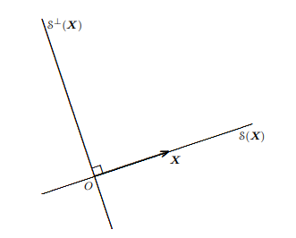
Figure $1.1$ illustrates the concepts discussed above for the case $n=2$ and $k=1$. The matrix of regressors $\boldsymbol{X}$ has only one column in this case, and it is therefore represented by a single vector in the figure. As a consequence, $\mathcal{S}(\boldsymbol{X})$ is one-dimensional, and since $n=2, \mathcal{S}^{\perp}(\boldsymbol{X})$ is also one-dimensional. Notice that $\mathcal{S}(\boldsymbol{X})$ and $\mathcal{S}^{\perp}(\boldsymbol{X})$ would be the same if $\boldsymbol{X}$ were any point on the straight line which is $\mathcal{S}(\boldsymbol{X})$, except for the origin. This illustrates the fact that $\mathcal{S}(\boldsymbol{X})$ is invariant to any nonsingular transformation of $\boldsymbol{X}$.
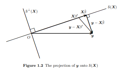
As we have seen, any point in $\mathcal{S}(\boldsymbol{X})$ can be represented by a vector of the form $\boldsymbol{X} \boldsymbol{\beta}$ for some $k$-vector $\boldsymbol{\beta}$. If one wants to find the point in $\mathcal{S}(\boldsymbol{X})$ that is closest to a given vector $\boldsymbol{y}$, the problem to be solved is that of minimizing, with respert tn the chnice of $\boldsymbol{\beta}$, the diktance hetween $\boldsymbol{y}$ and $\boldsymbol{X} \boldsymbol{\beta}$. Minimizing this distance is evidently equivalent to minimizing the square of this distance.
计量经济学代考
经济代写|计量经济学作业代写Econometrics代考|Introduction
计量经济学中最常用且在许多方面最重要的估计技术是最小二乘法。区分两种最小二乘、普通最小二乘或 OLS 和非线性最小二乘或 NLS 是有用的。在 OLS 的情况下,要估计的回归方程在所有参数上都是线性的,而在 NLS 的情况下,它至少在一个参数上是非线性的。OLS 估计可以通过几种不同的方式直接计算获得(见第 1.5 节),而 NLS 估计需要迭代过程(见第 6 章)。在本章中,我们将只讨论普通的最小二乘,因为理解线性回归对于理解本书中的其他内容至关重要。
使用 OLS 获得的估计值的数值和统计特性之间存在重要区别。数值属性是由于使用普通最小二乘而保持的属性,无论数据是如何生成的。由于这些属性是数值的,它们总是可以通过直接计算来验证。一个例子是众所周知的事实,即当回归量包含常数项时,OLS 残差总和为零。另一方面,统计属性是那些仅在关于数据生成方式的某些假设下才成立的属性。这些永远无法准确验证,尽管在某些情况下可以对其进行测试。一个例子是众所周知的命题,即 OLS 估计在某些情况下是无偏的。
数值属性和统计属性之间的区别显然是基本的。为了尽可能清楚地区分这种区别,我们将在本章中只讨论前者。我们将纯粹将普通最小二乘法作为一种计算工具来研究,而不会正式引入任何类型的统计模型(尽管我们有时会讨论线性回归模型中主要感兴趣的量)。在第 2 章之前不会介绍统计模型,我们将在第 2 章开始讨论非线性回归模型,其中线性回归模型当然是一个特例。
说我们将 OLS 作为一种计算设备来研究,并不是说我们将讨论计算 OLS 估计值的计算机算法(尽管我们将在 1.5 节中有限地这样做)。相反,我们的意思是我们将讨论普通最小二乘的数值性质,特别是这些性质的几何解释。OLS 的所有数值属性都可以用欧几里得几何来解释。在有限维向量空间的背景下,这种几何解释通常非常简单,只涉及毕达哥拉斯定理和高中三角学。然而,从这种方法中获得的洞察力非常好。一旦彻底掌握了普通最小二乘法所涉及的几何学,一个简单的几何论证通常可以为自己省去许多乏味的代数行。此外,正如我们希望本书的其余部分将说明的那样,理解 OLS 的几何特性对于理解所有类型的非线性模型和理解线性回归模型一样重要。
经济代写|计量经济学作业代写Econometrics代考|The Geometry of Least Squares
线性回归的基本成分是回归和是和回归矩阵X≡[X1…Xķ]. 倒数是是一个n-vector 和回归矩阵X是一个n×ķ矩阵,每一列X一世其中是一个n-向量。倒数是和每个回归器X1通过Xķ可以被认为是点n维欧几里得空间,和n. 这ķ回归量,只要它们是线性独立的,跨越ķ-维子空间和n. 我们将这个子空间表示为小号(X).1
子空间小号(X)由所有点组成和在和n这样和=XC总而言之C, 在哪里C是一个ķ=矢量。严格来说,我们应该指小号(X)作为由的列跨越的子空间X,但不太正式地,我们通常将其简单地称为跨度X. 的维度小号(X)总是等于ρ(X), 的等级X(即,列数X是线性独立的)。我们将假设ķ严格小于n,这在几乎所有实际情况下都是合理的。如果n小于ķ, 这将是不可能的X具有完整的列排名ķ.
如果不定义内积,就无法定义欧几里得空间。在这种情况下,我们感兴趣的内积就是所谓的自然内积。中任意两点的自然内积和n, 说和一世和和j, 可以表示⟨和一世,和j⟩并且定义为
⟨和一世,和j⟩≡∑吨=1n和一世吨和j吨≡和一世⊤和j≡和j⊤和一世
1 符号小号(X)不是标准的,没有我们喜欢的标准符号。我们相信这个符号有很多值得推荐的地方,因此以后会使用它。
经济代写|计量经济学作业代写Econometrics代考|The spaces S(X) and S⊥(X)
这是通过连接点来完成的和与原点并把箭头放在和. 然后,生成的箭头以图形方式显示有关向量的两个重要方面,即它的长度和方向。向量的欧几里得长度和是
|和|≡(∑吨=1n和吨2)1/2=|(和⊤和)1/2|
其中符号强调|和|是平方元素之和的正平方根和. 方向是向量本身归一化为长度单位,即和/|和|. 这种约定的一个优点是,如果我们移动其中一个箭头,注意既不改变它的长度也不改变它的方向,新的箭头表示相同的向量,即使箭头现在位于不同的点。这样做通常会非常方便,因此我们在大多数图表中都采用了这种约定。
数字1.1说明上述案例中讨论的概念n=2和ķ=1. 回归矩阵X在这种情况下只有一列,因此在图中用单个向量表示。作为结果,小号(X)是一维的,因为n=2,小号⊥(X)也是一维的。请注意小号(X)和小号⊥(X)如果X是直线上的任何一点小号(X),除了原点。这说明了一个事实小号(X)对任何非奇异变换是不变的X.
正如我们所见,任何一点小号(X)可以用以下形式的向量表示Xb对于一些ķ-向量b. 如果一个人想在小号(X)最接近给定向量的是, 要解决的问题是最小化, 对应的 chniceb, 之间的距离是和Xb. 最小化这个距离显然等同于最小化这个距离的平方。

统计代写请认准statistics-lab™. statistics-lab™为您的留学生涯保驾护航。
随机过程代考
在概率论概念中,随机过程是随机变量的集合。 若一随机系统的样本点是随机函数,则称此函数为样本函数,这一随机系统全部样本函数的集合是一个随机过程。 实际应用中,样本函数的一般定义在时间域或者空间域。 随机过程的实例如股票和汇率的波动、语音信号、视频信号、体温的变化,随机运动如布朗运动、随机徘徊等等。
贝叶斯方法代考
贝叶斯统计概念及数据分析表示使用概率陈述回答有关未知参数的研究问题以及统计范式。后验分布包括关于参数的先验分布,和基于观测数据提供关于参数的信息似然模型。根据选择的先验分布和似然模型,后验分布可以解析或近似,例如,马尔科夫链蒙特卡罗 (MCMC) 方法之一。贝叶斯统计概念及数据分析使用后验分布来形成模型参数的各种摘要,包括点估计,如后验平均值、中位数、百分位数和称为可信区间的区间估计。此外,所有关于模型参数的统计检验都可以表示为基于估计后验分布的概率报表。
广义线性模型代考
广义线性模型(GLM)归属统计学领域,是一种应用灵活的线性回归模型。该模型允许因变量的偏差分布有除了正态分布之外的其它分布。
statistics-lab作为专业的留学生服务机构,多年来已为美国、英国、加拿大、澳洲等留学热门地的学生提供专业的学术服务,包括但不限于Essay代写,Assignment代写,Dissertation代写,Report代写,小组作业代写,Proposal代写,Paper代写,Presentation代写,计算机作业代写,论文修改和润色,网课代做,exam代考等等。写作范围涵盖高中,本科,研究生等海外留学全阶段,辐射金融,经济学,会计学,审计学,管理学等全球99%专业科目。写作团队既有专业英语母语作者,也有海外名校硕博留学生,每位写作老师都拥有过硬的语言能力,专业的学科背景和学术写作经验。我们承诺100%原创,100%专业,100%准时,100%满意。
机器学习代写
随着AI的大潮到来,Machine Learning逐渐成为一个新的学习热点。同时与传统CS相比,Machine Learning在其他领域也有着广泛的应用,因此这门学科成为不仅折磨CS专业同学的“小恶魔”,也是折磨生物、化学、统计等其他学科留学生的“大魔王”。学习Machine learning的一大绊脚石在于使用语言众多,跨学科范围广,所以学习起来尤其困难。但是不管你在学习Machine Learning时遇到任何难题,StudyGate专业导师团队都能为你轻松解决。
多元统计分析代考
基础数据: $N$ 个样本, $P$ 个变量数的单样本,组成的横列的数据表
变量定性: 分类和顺序;变量定量:数值
数学公式的角度分为: 因变量与自变量
时间序列分析代写
随机过程,是依赖于参数的一组随机变量的全体,参数通常是时间。 随机变量是随机现象的数量表现,其时间序列是一组按照时间发生先后顺序进行排列的数据点序列。通常一组时间序列的时间间隔为一恒定值(如1秒,5分钟,12小时,7天,1年),因此时间序列可以作为离散时间数据进行分析处理。研究时间序列数据的意义在于现实中,往往需要研究某个事物其随时间发展变化的规律。这就需要通过研究该事物过去发展的历史记录,以得到其自身发展的规律。
回归分析代写
多元回归分析渐进(Multiple Regression Analysis Asymptotics)属于计量经济学领域,主要是一种数学上的统计分析方法,可以分析复杂情况下各影响因素的数学关系,在自然科学、社会和经济学等多个领域内应用广泛。
MATLAB代写
MATLAB 是一种用于技术计算的高性能语言。它将计算、可视化和编程集成在一个易于使用的环境中,其中问题和解决方案以熟悉的数学符号表示。典型用途包括:数学和计算算法开发建模、仿真和原型制作数据分析、探索和可视化科学和工程图形应用程序开发,包括图形用户界面构建MATLAB 是一个交互式系统,其基本数据元素是一个不需要维度的数组。这使您可以解决许多技术计算问题,尤其是那些具有矩阵和向量公式的问题,而只需用 C 或 Fortran 等标量非交互式语言编写程序所需的时间的一小部分。MATLAB 名称代表矩阵实验室。MATLAB 最初的编写目的是提供对由 LINPACK 和 EISPACK 项目开发的矩阵软件的轻松访问,这两个项目共同代表了矩阵计算软件的最新技术。MATLAB 经过多年的发展,得到了许多用户的投入。在大学环境中,它是数学、工程和科学入门和高级课程的标准教学工具。在工业领域,MATLAB 是高效研究、开发和分析的首选工具。MATLAB 具有一系列称为工具箱的特定于应用程序的解决方案。对于大多数 MATLAB 用户来说非常重要,工具箱允许您学习和应用专业技术。工具箱是 MATLAB 函数(M 文件)的综合集合,可扩展 MATLAB 环境以解决特定类别的问题。可用工具箱的领域包括信号处理、控制系统、神经网络、模糊逻辑、小波、仿真等。