如果你也在 怎样代写多元统计分析Multivariate Statistical Analysis这个学科遇到相关的难题，请随时右上角联系我们的24/7代写客服。

多元统计分析被认为是评估地球化学异常与任何单独变量和变量之间相互影响的意义的有用工具。

statistics-lab™ 为您的留学生涯保驾护航 在代写多元统计分析Multivariate Statistical Analysis方面已经树立了自己的口碑, 保证靠谱, 高质且原创的统计Statistics代写服务。我们的专家在代写多元统计分析Multivariate Statistical Analysis代写方面经验极为丰富，各种代写多元统计分析Multivariate Statistical Analysis相关的作业也就用不着说。

我们提供的多元统计分析Multivariate Statistical Analysis及其相关学科的代写，服务范围广, 其中包括但不限于:

• Statistical Inference 统计推断
• Statistical Computing 统计计算
• Advanced Probability Theory 高等概率论
• Advanced Mathematical Statistics 高等数理统计学
• (Generalized) Linear Models 广义线性模型
• Statistical Machine Learning 统计机器学习
• Longitudinal Data Analysis 纵向数据分析
• Foundations of Data Science 数据科学基础

统计代写|多元统计分析代写Multivariate Statistical Analysis代考|Reliability of Systems

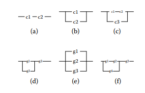
Consider a system, comprising components $c_{1}, \ldots, c_{n}$, and let $p_{j}$ be the reliability of component $c_{j}$, that is, its probability of being $u p$ (in working order). We wish to calculate the reliability $R$ of the whole system from the component reliabilities. It is assumed throughout that the components operate independently.
Example

1. Series system: this is shown in Figure 2.1a. Since the system can operate only if both components are up, the reliability is
   $$
   R=\mathrm{P}\left(c_{1} u p \text { and } c_{2} u p\right)=\mathrm{P}\left(c_{1} u p\right) \times \mathrm{P}\left(c_{2} u p\right)=p_{1} p_{2}
   $$
   using the independence of $c_{1}$ and $c_{2}$.
2. Parallel system: this is shown in Figure $2.1 \mathrm{~b}$. The system can operate if either $c_{1}$ or $c_{2}$ is up, so
   $$
   \begin{aligned}
   R &=1-\mathrm{P}\left(c_{1} \text { down and } c_{2} \text { down }\right) \
   &=1-\mathrm{P}\left(c_{1} \text { down }\right) \times \mathrm{P}\left(c_{2} \text { down }\right)=1-\left(1-p_{1}\right)\left(1-p_{2}\right)
   \end{aligned}
   $$
   This can easily be extended to $n$ components: for a series system $R=$ $p_{1} p_{2} \ldots p_{n}$, and for a parallel system $R=1-\left(1-p_{1}\right)\left(1-p_{2}\right) \ldots\left(1-p_{n}\right)$. Further, components can be replaced by subsystems in more complex systems and networks.

统计代写|多元统计分析代写Multivariate Statistical Analysis代考|Stress and Strength

Suppose that a system (electronic, mechanical, chemical, biological) has strength $X$ on some scale that measures its resistance to failure. The system will have been constructed or assembled to some nominal strength specification, say $\mu_{X} ;$ but in practice, $X$ will be randomly distributed around $\mu_{X}$. Once in operation, suppose that the system will be exposed to stress $Y$ randomly distributed around some level $\mu_{Y}$. The system will fail if $X<Y$, and we are interested in the probability of this event.
Let $f(x, y)$ be the joint density of $X$ and $Y$, then
$$
\mathrm{P}(\text { failure })=\mathrm{P}(X<Y)=\int_{x<y} f(x, y) d x d y=\int_{0}^{\infty} d x \int_{x}^{\infty} d y{f(x, y)}
$$
If, as is usual, $X$ and $Y$ are independent, $f(x, y)=f_{X}(x) f_{Y}(y)$, and then
$$
\mathrm{P}(X<Y)=\int_{0}^{\infty} d x \int_{x}^{\infty} d y\left{f_{X}(x) f_{Y}(y)\right}=\int_{0}^{\infty} f_{X}(x)\left{1-F_{Y}(x)\right} d x
$$
where $F_{Y}$ is the distribution function of $Y$. Equivalently,
$$
\mathrm{P}(X<Y)=\int_{0}^{\infty} d y \int_{0}^{y} d x{f(x, y)}=\int_{0}^{\infty} f_{Y}(y) F_{X}(y) d y .
$$
In the survival version of the situation, $X$ and $Y$ may vary over time, and then we have $X(t)$ and $Y(t)$. The system will fail at time $s$ if $X(t) \geq Y(t)$ for $0 \leq t<s$, and $X(s)<Y(s)$. The forms taken by $X(t)$ and $Y(t)$ can vary widely between different applications; for example, $X(t)$ might be constant or steadily decreasing over time, and $Y(t)$ might be constant, steadily increasing, randomly fluctuating, or result from intermittent shocks to the system. The analysis in such cases can be quite difficult: $T$ is the first time at which the stochastic process $X(t)-Y(t)$ becomes negative.

统计代写|多元统计分析代写Multivariate Statistical Analysis代考|Survival Distributions

1. Derive the density $f(t)=\xi^{-1} \mathrm{e}^{-t / \xi}$ of the exponential distribution and show that its mean is $\xi$ and that its variance is $\xi^{2}$. Prove the lack-of-memory property. What is the distribution of $(T / \xi)^{v}$ for $v>0$ ? What about $v<0$ ?
2. Derive the mean and variance of the Weibull distribution. Verify that the upper $q$ th quantile is $t_{q}=\xi(-\log q)^{1 / v}$.
3. Suppose that $Y$ has distribution $N\left(\mu, \sigma^{2}\right)$ and that $T=\mathrm{e}^{Y}$ : then $T$ has a log-normal distribution. Confirm that $\mathrm{E}\left(T^{r}\right)=\mathrm{e}^{r \mu+\sigma^{2} / 2}$. Derive the mean and variance of $T$ as $\mu_{T}=\mathrm{E}(T)=\mathrm{e}^{\mu+\sigma^{2} / 2}$ and

$\sigma_{T}^{2}=\operatorname{var}(T)=\left(\mathrm{e}^{\sigma^{2}}-1\right) \mu_{T}^{2}$. Note that the survivor and hazard functions are not explicit, only expressible in terms of $\Phi$, the standard normal distribution function.

4. Another generalisation of the exponential distribution is the gamma, which has density $f(t)=\Gamma(v)^{-1} \xi^{-v} t^{v-1} \mathrm{e}^{t / \xi}$. The parameters are $\xi>0$ (scale) and $v>0$ (shape); the exponential is recovered with $v=1$. Derive the survivor function as $\bar{F}(t)=1-\Gamma^{(r)}(v ; t / \xi)$, where $\Gamma^{(r)}(v ; z)=\Gamma(v)^{-1} \int_{0}^{z} y^{v-1} \mathrm{e}^{-y} d y$ is the incomplete gamma function ratio.
5. Calculate the mean, variance, and upper $100 q \%$ quantile of the Pareto distribution. Take care regarding the size of $\gamma$.
6. As a generalisation of the Pareto distribution, step up the Burr: this has survivor function $\bar{F}(t)=\left{1+(t / \alpha)^{\rho}\right}^{-\gamma}$, just replacing $t / \alpha$ by $(t / \alpha)^{\rho}$ with $\rho>0$. Derive its hazard function: is it IFR, DFR, or what? You might suspect that, by analogy with the derivation of the Pareto given above, the Burr can be mocked up as some sort of Weibullgamma combination. Can it? The special case $\gamma=1$ gives the loglogistic distribution.
7. Prove the following:
   a. If $\int_{0}^{\infty} h(t) d t<\infty$, then $\mathrm{P}(T=\infty)>0$.
   b. If $h(t)=h_{1}(t)+h_{2}(t)$, where $h_{1}(t)$ and $h_{2}(t)$ are the hazard functions of independent failure time variates $T_{1}$ and $T_{2}$, then $T$ has the same distribution as $\min \left(T_{1}, T_{2}\right)$.
8. Calculate $\mathrm{P}\left(T>t_{0}\right)$ and $\mathrm{P}\left(T>2 t_{0}\right)$ when $T$ has hazard function $h(t)=a$ for $0<t<t_{0}, h(t)=b$ for $t \geq t_{0}$.
9. Show that, for continuous $T, \mathrm{E}(T)=\int_{0}^{\infty} \bar{F}(t) d t$, provided that $t \bar{F}(t) \rightarrow$ 0 as $t \rightarrow \infty$. For discrete $T$, taking values $0,1, \ldots$ with probabilities $p_{0}, p_{1}, \ldots$, let $q_{j}=\mathrm{P}(T>j)$ : show that $\mathrm{E}(T)=\sum_{j=1}^{\infty} q_{j}$.
10. Negative binomial distribution: verify that the probabilities $p_{r}=$ $\left(\begin{array}{c}\kappa+r-1 \ \kappa-1\end{array}\right) \rho^{r}(1-\rho)^{\kappa}(r=0,1,2, \ldots)$ sum to $1 .$
11. Sometimes survival data are reduced to binary outcomes. Thus, all that is recorded is whether $T>t^{}$ or not, where $t^{}$ is some threshold, for example, five-year survival after cancer treatment. For Weibull lifetimes $p^{}=\mathrm{P}\left(T>t^{}\right)=\exp \left{-\left(t^{} / \xi\right)^{v}\right}$, solog $\left(-\log p^{}\right)=v \log t^{}-$ $v \log \xi .$ A log-linear regression model for $\xi$ then gives a complementary $\log -\log$ form for $p^{}: \log \left(-\log p^{*}\right)=\beta_{0}+\mathbf{x}^{T} \beta$. What lifetime distribution corresponds to a logit-linear model for binary data?

多元统计分析代写

统计代写|多元统计分析代写Multivariate Statistical Analysis代考|Reliability of Systems

考虑一个系统，包括组件C1,…,Cn， 然后让pj是组件的可靠性Cj，也就是它出现的概率在p（按工作顺序）。我们希望计算可靠性R整个系统从组件的可靠性。始终假定组件独立运行。
例子

1. 串联系统：如图 2.1a 所示。由于系统只有在两个组件都启动时才能运行，因此可靠性是
   R=磷(C1在p 和 C2在p)=磷(C1在p)×磷(C2在p)=p1p2
   使用独立性C1和C2.
2. 并联系统：如图所示2.1 b. 系统可以运行，如果C1或者C2起来了，所以
   R=1−磷(C1 下来和 C2 向下 ) =1−磷(C1 向下 )×磷(C2 向下 )=1−(1−p1)(1−p2)
   这可以很容易地扩展到n组件：用于串联系统R= p1p2…pn, 对于并行系统R=1−(1−p1)(1−p2)…(1−pn). 此外，组件可以被更复杂的系统和网络中的子系统替换。

统计代写|多元统计分析代写Multivariate Statistical Analysis代考|Stress and Strength

假设一个系统（电子、机械、化学、生物）具有强度X在某种程度上衡量其对失败的抵抗力。该系统将按照某些标称强度规格构建或组装，例如μX;但在实践中，X会随机分布在μX. 一旦投入运行，假设系统将承受压力是随机分布在某个级别μ是. 系统将失败，如果X<是，我们对这个事件的概率感兴趣。
让F(X,是)是联合密度X和是， 然后
磷( 失败 )=磷(X<是)=∫X<是F(X,是)dXd是=∫0∞dX∫X∞d是F(X,是)
如果像往常一样，X和是是独立的，F(X,是)=FX(X)F是(是)， 进而
\mathrm{P}(X<Y)=\int_{0}^{\infty} d x \int_{x}^{\infty} d y\left{f_{X}(x) f_{Y}(y) \right}=\int_{0}^{\infty} f_{X}(x)\left{1-F_{Y}(x)\right} d x\mathrm{P}(X<Y)=\int_{0}^{\infty} d x \int_{x}^{\infty} d y\left{f_{X}(x) f_{Y}(y) \right}=\int_{0}^{\infty} f_{X}(x)\left{1-F_{Y}(x)\right} d x
在哪里F是是分布函数是. 等效地，
磷(X<是)=∫0∞d是∫0是dXF(X,是)=∫0∞F是(是)FX(是)d是.
在生存版的情况下，X和是可能会随着时间而变化，然后我们有X(吨)和是(吨). 系统会及时失效s如果X(吨)≥是(吨)为了0≤吨<s， 和X(s)<是(s). 采取的形式X(吨)和是(吨)在不同的应用程序之间可以有很大的不同；例如，X(吨)可能会随着时间的推移保持不变或稳步下降，并且是(吨)可能是恒定的、稳定增加的、随机波动的，或者是系统受到间歇性冲击的结果。在这种情况下进行分析可能非常困难：吨是随机过程的第一次X(吨)−是(吨)变成负数。

统计代写|多元统计分析代写Multivariate Statistical Analysis代考|Survival Distributions

1. 导出密度F(吨)=X−1和−吨/X的指数分布，并证明它的平均值是X并且它的方差是X2. 证明内存不足的性质。什么是分布(吨/X)在为了在>0? 关于什么在<0 ?
2. 导出 Weibull 分布的均值和方差。验证上层q第分位数是吨q=X(−日志⁡q)1/在.
3. 假设是有分布ñ(μ,σ2)然后吨=和是： 然后吨具有对数正态分布。确认这个和(吨r)=和rμ+σ2/2. 导出均值和方差吨作为μ吨=和(吨)=和μ+σ2/2和

σ吨2=曾是⁡(吨)=(和σ2−1)μ吨2. 请注意，幸存者和危险函数不是明确的，只能表示为披，标准正态分布函数。

4. 指数分布的另一个推广是 gamma，它具有密度F(吨)=Γ(在)−1X−在吨在−1和吨/X. 参数是X>0（规模）和在>0（形状）; 指数恢复为在=1. 导出幸存者函数为F¯(吨)=1−Γ(r)(在;吨/X)， 在哪里Γ(r)(在;和)=Γ(在)−1∫0和是在−1和−是d是是不完全伽马函数比。
5. 计算均值、方差和上限100q%帕累托分布的分位数。注意大小C.
6. 作为帕累托分布的推广，加强毛刺：这具有幸存者功能\bar{F}(t)=\left{1+(t / \alpha)^{\rho}\right}^{-\gamma}\bar{F}(t)=\left{1+(t / \alpha)^{\rho}\right}^{-\gamma}, 只是替换吨/一种经过(吨/一种)ρ和ρ>0. 推导出它的危险函数：是 IFR、DFR 还是什么？您可能会怀疑，通过与上面给出的 Pareto 推导类比，Burr 可以模拟为某种 Weibullgamma 组合。它可以？特殊情况C=1给出对数逻辑分布。
7. 证明以下几点
   ：如果∫0∞H(吨)d吨<∞， 然后磷(吨=∞)>0.
   湾。如果H(吨)=H1(吨)+H2(吨)， 在哪里H1(吨)和H2(吨)是独立失效时间变量的危险函数吨1和吨2， 然后吨具有相同的分布分钟(吨1,吨2).
8. 计算磷(吨>吨0)和磷(吨>2吨0)什么时候吨具有危险功能H(吨)=一种为了0<吨<吨0,H(吨)=b为了吨≥吨0.
9. 证明，对于连续吨,和(吨)=∫0∞F¯(吨)d吨, 前提是吨F¯(吨)→0 为吨→∞. 对于离散吨, 取值0,1,…有概率p0,p1,…， 让qj=磷(吨>j)： 显示和(吨)=∑j=1∞qj.
10. 负二项分布：验证概率pr= (ķ+r−1 ķ−1)ρr(1−ρ)ķ(r=0,1,2,…)总和1.
11. 有时生存数据被简化为二元结果。因此，记录的只是是否吨>吨与否，在哪里吨是一些阈值，例如，癌症治疗后的五年生存率。威布尔一生p^{}=\mathrm{P}\left(T>t^{}\right)=\exp \left{-\left(t^{} / \xi\right)^{v}\right}p^{}=\mathrm{P}\left(T>t^{}\right)=\exp \left{-\left(t^{} / \xi\right)^{v}\right}, 独奏(−日志⁡p)=在日志⁡吨− 在日志⁡X.对数线性回归模型X然后给出一个互补的日志−日志表格p:日志⁡(−日志⁡p∗)=b0+X吨b. 什么寿命分布对应于二进制数据的 logit 线性模型？

统计代写请认准statistics-lab™. statistics-lab™为您的留学生涯保驾护航。

金融工程代写

金融工程是使用数学技术来解决金融问题。金融工程使用计算机科学、统计学、经济学和应用数学领域的工具和知识来解决当前的金融问题，以及设计新的和创新的金融产品。

非参数统计代写

非参数统计指的是一种统计方法，其中不假设数据来自于由少数参数决定的规定模型；这种模型的例子包括正态分布模型和线性回归模型。

广义线性模型代考

广义线性模型（GLM）归属统计学领域，是一种应用灵活的线性回归模型。该模型允许因变量的偏差分布有除了正态分布之外的其它分布。

术语 广义线性模型（GLM）通常是指给定连续和/或分类预测因素的连续响应变量的常规线性回归模型。它包括多元线性回归，以及方差分析和方差分析（仅含固定效应）。

有限元方法代写

有限元方法（FEM）是一种流行的方法，用于数值解决工程和数学建模中出现的微分方程。典型的问题领域包括结构分析、传热、流体流动、质量运输和电磁势等传统领域。

有限元是一种通用的数值方法，用于解决两个或三个空间变量的偏微分方程（即一些边界值问题）。为了解决一个问题，有限元将一个大系统细分为更小、更简单的部分，称为有限元。这是通过在空间维度上的特定空间离散化来实现的，它是通过构建对象的网格来实现的：用于求解的数值域，它有有限数量的点。边界值问题的有限元方法表述最终导致一个代数方程组。该方法在域上对未知函数进行逼近。[1] 然后将模拟这些有限元的简单方程组合成一个更大的方程系统，以模拟整个问题。然后，有限元通过变化微积分使相关的误差函数最小化来逼近一个解决方案。

tatistics-lab作为专业的留学生服务机构，多年来已为美国、英国、加拿大、澳洲等留学热门地的学生提供专业的学术服务，包括但不限于Essay代写，Assignment代写，Dissertation代写，Report代写，小组作业代写，Proposal代写，Paper代写，Presentation代写，计算机作业代写，论文修改和润色，网课代做，exam代考等等。写作范围涵盖高中，本科，研究生等海外留学全阶段，辐射金融，经济学，会计学，审计学，管理学等全球99%专业科目。写作团队既有专业英语母语作者，也有海外名校硕博留学生，每位写作老师都拥有过硬的语言能力，专业的学科背景和学术写作经验。我们承诺100%原创，100%专业，100%准时，100%满意。

随机分析代写

随机微积分是数学的一个分支，对随机过程进行操作。它允许为随机过程的积分定义一个关于随机过程的一致的积分理论。这个领域是由日本数学家伊藤清在第二次世界大战期间创建并开始的。

时间序列分析代写

随机过程，是依赖于参数的一组随机变量的全体，参数通常是时间。 随机变量是随机现象的数量表现，其时间序列是一组按照时间发生先后顺序进行排列的数据点序列。通常一组时间序列的时间间隔为一恒定值（如1秒，5分钟，12小时，7天，1年），因此时间序列可以作为离散时间数据进行分析处理。研究时间序列数据的意义在于现实中，往往需要研究某个事物其随时间发展变化的规律。这就需要通过研究该事物过去发展的历史记录，以得到其自身发展的规律。

回归分析代写

多元回归分析渐进（Multiple Regression Analysis Asymptotics）属于计量经济学领域，主要是一种数学上的统计分析方法，可以分析复杂情况下各影响因素的数学关系，在自然科学、社会和经济学等多个领域内应用广泛。

MATLAB代写

MATLAB 是一种用于技术计算的高性能语言。它将计算、可视化和编程集成在一个易于使用的环境中，其中问题和解决方案以熟悉的数学符号表示。典型用途包括：数学和计算算法开发建模、仿真和原型制作数据分析、探索和可视化科学和工程图形应用程序开发，包括图形用户界面构建MATLAB 是一个交互式系统，其基本数据元素是一个不需要维度的数组。这使您可以解决许多技术计算问题，尤其是那些具有矩阵和向量公式的问题，而只需用 C 或 Fortran 等标量非交互式语言编写程序所需的时间的一小部分。MATLAB 名称代表矩阵实验室。MATLAB 最初的编写目的是提供对由 LINPACK 和 EISPACK 项目开发的矩阵软件的轻松访问，这两个项目共同代表了矩阵计算软件的最新技术。MATLAB 经过多年的发展，得到了许多用户的投入。在大学环境中，它是数学、工程和科学入门和高级课程的标准教学工具。在工业领域，MATLAB 是高效研究、开发和分析的首选工具。MATLAB 具有一系列称为工具箱的特定于应用程序的解决方案。对于大多数 MATLAB 用户来说非常重要，工具箱允许您学习和应用专业技术。工具箱是 MATLAB 函数（M 文件）的综合集合，可扩展 MATLAB 环境以解决特定类别的问题。可用工具箱的领域包括信号处理、控制系统、神经网络、模糊逻辑、小波、仿真等。

R语言代写	问卷设计与分析代写
PYTHON代写	回归分析与线性模型代写
MATLAB代写	方差分析与试验设计代写
STATA代写	机器学习/统计学习代写
SPSS代写	计量经济学代写
EVIEWS代写	时间序列分析代写
EXCEL代写	深度学习代写
SQL代写	各种数据建模与可视化代写