如果你也在 怎样代写多元统计分析Multivariate Statistical Analysis这个学科遇到相关的难题,请随时右上角联系我们的24/7代写客服。
多变量统计分析被认为是评估地球化学异常与任何单独变量和变量之间相互影响的意义的有用工具。
statistics-lab™ 为您的留学生涯保驾护航 在代写多元统计分析Multivariate Statistical Analysis方面已经树立了自己的口碑, 保证靠谱, 高质且原创的统计Statistics代写服务。我们的专家在代写多元统计分析Multivariate Statistical Analysis代写方面经验极为丰富,各种代写多元统计分析Multivariate Statistical Analysis相关的作业也就用不着说。
我们提供的多元统计分析Multivariate Statistical Analysis及其相关学科的代写,服务范围广, 其中包括但不限于:
- Statistical Inference 统计推断
- Statistical Computing 统计计算
- Advanced Probability Theory 高等概率论
- Advanced Mathematical Statistics 高等数理统计学
- (Generalized) Linear Models 广义线性模型
- Statistical Machine Learning 统计机器学习
- Longitudinal Data Analysis 纵向数据分析
- Foundations of Data Science 数据科学基础
统计代写|多元统计分析代写Multivariate Statistical Analysis代考|Multivariate Laplace Distribution
Let $g$ and $G$ be the pdf and cdf of a $d$-dimensional Gaussian distribution $N_{d}(0, \Sigma)$, the pdf and cdf of a multivariate Laplace distribution can be written as
$f_{M \text { Laplace } d}(x ; m, \Sigma)=\int_{0}^{\infty} g\left(z^{-\frac{1}{2}} x-z^{\frac{1}{2}} m\right) z^{-\frac{d}{2}} e^{-z} d z$
$F_{M \text { Laplace }{d}}(x, m, \Sigma)=\int{0}^{\infty} G\left(z^{-\frac{1}{2}} x-z^{\frac{1}{2}} m\right) e^{-z} d z$
the pdf can also be described as
$$
\begin{aligned}
f_{M \text { Laplace }{d}}(x ; m, \Sigma)=& \frac{2 e^{x^{\top} \Sigma^{-1} m}}{(2 \pi)^{\frac{d}{2}}|\Sigma|^{\frac{1}{2}}}\left(\frac{x^{\top} \Sigma^{-1} x}{2+m^{\top} \Sigma^{-1} m}\right)^{\frac{2}{2}} \ & \times K{\lambda}\left(\sqrt{\left(2+m^{\top} \Sigma^{-1} m\right)\left(x^{\top} \Sigma^{-1} x\right)}\right)
\end{aligned}
$$
where $\lambda=\frac{2-d}{2}$ and $K_{\lambda}(x)$ is the modified Bessel function of the third kind
$$
K_{\lambda}(x)=\frac{1}{2}\left(\frac{x}{2}\right)^{\lambda} \int_{0}^{\infty} t^{-\lambda-1} e^{-t-\frac{t^{2}}{4 t}} d t, \quad x>0
$$
Multivariate Laplace distribution has mean and variance
$$
\begin{aligned}
\mathrm{E}[X] &=m \
\operatorname{Cov}[X] &=\Sigma+m m^{\top}
\end{aligned}
$$
统计代写|多元统计分析代写Multivariate Statistical Analysis代考|Copulae
The cumulative distribution function (cdf) of a two-dimensional vector $\left(X_{1}, X_{2}\right)$ is given by
$$
F\left(x_{1}, x_{2}\right)=\mathrm{P}\left(X_{1} \leq x_{1}, X_{2} \leq x_{2}\right)
$$
For the case that $X_{1}$ and $X_{2}$ are independent, their joint cumulative distribution function $F\left(x_{1}, x_{2}\right)$ can be written as a product of their one-dimensional marginals:
$$
F\left(x_{1}, x_{2}\right)=F_{X_{1}}\left(x_{1}\right) F_{X_{2}}\left(x_{2}\right)=\mathrm{P}\left(X_{1} \leq x_{1}\right) \mathrm{P}\left(X_{2} \leq x_{2}\right) .
$$
But how can we model dependence of $X_{1}$ and $X_{2}$ ? Most people would suggest linear correlation. Correlation is though an appropriate measure of dependence only when the random variables have an elliptical or spherical distribution, which include the normal multivariate distribution. Although the terms “correlation” and “dependency” are often used interchangeably, correlation is actually a rather imperfect measure of dependency, and there are many circumstances where correlation should not be used.
Copulae represent an elegant concept of connecting marginals with joint cumulative distribution functions. Copulae are functions that join or “couple” multivariate distribution functions to their one-dimensional marginal distribution functions. Let us consider a $d$-dimensional vector $X=\left(X_{1}, \ldots, X_{d}\right)^{\top}$. Using copulae, the marginal distribution functions $F_{X_{i}}(i=1, \ldots, d)$ can be separately modelled from their dependence structure and then coupled together to form the multivariate distribution $F_{X}$. Copula functions have a long history in probability theory and statistics. Their application in finance is very recent. Copulae are important in Valueat-Risk calculations and constitute an essential tool in quantitative finance (Härdle et al., 2009).
First let us concentrate on the two-dimensional case, then we will extend this concept to the $d$-dimensional case, for a random variable in $\mathbb{R}^{d}$ with $d \geq 1$. To be able to define a copula function, first we need to represent a concept of the volume of a rectangle, a 2 -increading function and a grounded function.
Let $U_{1}$ and $U_{2}$ be two sets in $\overline{\mathbb{R}}=\mathbb{R} \cup{+\infty} \cup{-\infty}$ and consider the function $F: U_{1} \times U_{2} \longrightarrow \mathbb{\mathbb { R }}$.
统计代写|多元统计分析代写Multivariate Statistical Analysis代考|Elementary Properties of the Multinormal
Let us first summarise some properties which were already derived in the previous chapter.
- The pdf of $X \sim N_{p}(\mu, \Sigma)$ is
$$
f(x)=|2 \pi \Sigma|^{-1 / 2} \exp \left{-\frac{1}{2}(x-\mu)^{\top} \Sigma^{-1}(x-\mu)\right}
$$
The expectation is $\mathrm{E}(X)=\mu$, the covariance can be calculated as $\operatorname{Var}(X)=\mathrm{E}(X-\mu)(X-\mu)^{\top}=\Sigma$.
Linear transformations turn normal random variables into normal random variables. If $X \sim N_{p}(\mu, \Sigma)$ and $\mathcal{A}(p \times p), c \in \mathbb{R}^{p}$, then $Y=\mathcal{A} X+c$ is $p$-variate Normal, i.e.
$$
Y \sim N_{p}\left(\mathcal{A} \mu+c, \mathcal{A} \Sigma \cdot \mathcal{A}^{\top}\right)
$$
If $X \sim N_{p}(\mu, \Sigma)$, then the Mahalanobis transformation is
$$
Y=\Sigma^{-1 / 2}(X-\mu) \sim N_{p}\left(0, \mathcal{I}{p}\right) $$ and it holds that $$ Y^{\top} Y=(X-\mu)^{\top} \Sigma^{-1}(X-\mu) \sim \chi{p}^{2}
$$
Often it is interesting to partition $X$ into sub-vectors $X_{1}$ and $X_{2}$. The following theorem tells us how to correct $X_{2}$ to obtain a vector which is independent of $X_{1}$.
Theorem 5.1 Let $X=\left(\begin{array}{l}X_{1} \ X_{2}\end{array}\right) \sim N_{p}(\mu, \Sigma), X_{1} \in \mathbb{R}^{r}, X_{2} \in \mathbb{R}^{p-r}$. Define $X_{2.1}=$ $X_{2}-\Sigma_{21} \Sigma_{11}^{-1} X_{1}$ from the partitioned covariance matrix
$$
\Sigma=\left(\begin{array}{cc}
\Sigma_{11} & \Sigma_{12} \
\Sigma_{21} & \Sigma_{22}
\end{array}\right)
$$
Then
$$
\begin{array}{r}
X_{1} \sim N_{r}\left(\mu_{1}, \Sigma_{11}\right), \
X_{2.1} \sim N_{p-r}\left(\mu_{2.1}, \Sigma_{22.1}\right)
\end{array}
$$
are independent with
$$
\mu_{2.1}=\mu_{2}-\Sigma_{21} \Sigma_{11}^{-1} \mu_{1}, \quad \Sigma_{22.1}=\Sigma_{22}-\Sigma_{21} \Sigma_{11}^{-1} \Sigma_{12}
$$
Proof
$$
\begin{array}{rlll}
X_{1} & =\mathcal{A} X & \text { with } & \mathcal{A}=\left(\mathcal{I}{r}, 0\right) \ X{2.1} & =\mathcal{B} X & \text { with } & \mathcal{B}=\left(-\Sigma_{21} \Sigma_{11}^{-1}, \mathcal{I}_{p-r}\right)
\end{array}
$$
多元统计分析代考
统计代写|多元统计分析代写Multivariate Statistical Analysis代考|Multivariate Laplace Distribution
让G和G成为 a 的 pdf 和 cdfd维高斯分布ñd(0,Σ), 多元拉普拉斯分布的 pdf 和 cdf 可以写成
F米 拉普拉斯 d(X;米,Σ)=∫0∞G(和−12X−和12米)和−d2和−和d和
F米 拉普拉斯 d(X,米,Σ)=∫0∞G(和−12X−和12米)和−和d和
pdf也可以描述为
F米 拉普拉斯 d(X;米,Σ)=2和X⊤Σ−1米(2圆周率)d2|Σ|12(X⊤Σ−1X2+米⊤Σ−1米)22 ×ķλ((2+米⊤Σ−1米)(X⊤Σ−1X))
在哪里λ=2−d2和ķλ(X)是第三类修正贝塞尔函数
ķλ(X)=12(X2)λ∫0∞吨−λ−1和−吨−吨24吨d吨,X>0
多元拉普拉斯分布具有均值和方差
和[X]=米 这[X]=Σ+米米⊤
统计代写|多元统计分析代写Multivariate Statistical Analysis代考|Copulae
二维向量的累积分布函数 (cdf)(X1,X2)是(谁)给的
F(X1,X2)=磷(X1≤X1,X2≤X2)
对于这种情况X1和X2是独立的,它们的联合累积分布函数F(X1,X2)可以写成它们的一维边际的乘积:
F(X1,X2)=FX1(X1)FX2(X2)=磷(X1≤X1)磷(X2≤X2).
但是我们如何模拟X1和X2? 大多数人会建议线性相关。仅当随机变量具有椭圆或球形分布(包括正态多元分布)时,相关性才是适当的相关性度量。尽管术语“相关性”和“依赖性”经常互换使用,但相关性实际上是一种相当不完善的依赖性度量,并且在许多情况下不应该使用相关性。
Copulae 代表了一个优雅的概念,它将边缘与联合累积分布函数连接起来。Copulae 是将多元分布函数连接或“耦合”到其一维边际分布函数的函数。让我们考虑一个d维向量X=(X1,…,Xd)⊤. 使用 copulae,边际分布函数FX一世(一世=1,…,d)可以从它们的依赖结构中单独建模,然后耦合在一起形成多元分布FX. Copula 函数在概率论和统计学中有着悠久的历史。它们在金融领域的应用是最近才出现的。Copulae 在 Valueat-Risk 计算中很重要,并且构成了量化金融中的重要工具(Härdle 等,2009)。
首先让我们专注于二维情况,然后我们将把这个概念扩展到d维情况,对于随机变量Rd和d≥1. 为了能够定义一个 copula 函数,首先我们需要表示一个矩形体积的概念,一个 2 递增函数和一个接地函数。
让在1和在2有两套R¯=R∪+∞∪−∞并考虑函数F:在1×在2⟶R.
统计代写|多元统计分析代写Multivariate Statistical Analysis代考|Elementary Properties of the Multinormal
让我们首先总结一些在前一章已经推导出来的性质。
- 的pdfX∼ñp(μ,Σ)是
f(x)=|2 \pi \Sigma|^{-1 / 2} \exp \left{-\frac{1}{2}(x-\mu)^{\top} \Sigma^{-1 }(x-\mu)\right}f(x)=|2 \pi \Sigma|^{-1 / 2} \exp \left{-\frac{1}{2}(x-\mu)^{\top} \Sigma^{-1 }(x-\mu)\right}
期望是和(X)=μ,协方差可以计算为曾是(X)=和(X−μ)(X−μ)⊤=Σ.
线性变换将正态随机变量转换为正态随机变量。如果X∼ñp(μ,Σ)和一个(p×p),C∈Rp, 然后是=一个X+C是p-variate Normal,即
是∼ñp(一个μ+C,一个Σ⋅一个⊤)
如果X∼ñp(μ,Σ),则马氏变换为
是=Σ−1/2(X−μ)∼ñp(0,我p)它认为
是⊤是=(X−μ)⊤Σ−1(X−μ)∼χp2
分区通常很有趣X成子向量X1和X2. 下面的定理告诉我们如何纠正X2获得一个独立于的向量X1.
定理 5.1 让X=(X1 X2)∼ñp(μ,Σ),X1∈Rr,X2∈Rp−r. 定义X2.1= X2−Σ21Σ11−1X1从分区协方差矩阵
Σ=(Σ11Σ12 Σ21Σ22)
然后
X1∼ñr(μ1,Σ11), X2.1∼ñp−r(μ2.1,Σ22.1)
独立于
μ2.1=μ2−Σ21Σ11−1μ1,Σ22.1=Σ22−Σ21Σ11−1Σ12
证明
X1=一个X 和 一个=(我r,0) X2.1=乙X 和 乙=(−Σ21Σ11−1,我p−r)

统计代写请认准statistics-lab™. statistics-lab™为您的留学生涯保驾护航。
金融工程代写
金融工程是使用数学技术来解决金融问题。金融工程使用计算机科学、统计学、经济学和应用数学领域的工具和知识来解决当前的金融问题,以及设计新的和创新的金融产品。
非参数统计代写
非参数统计指的是一种统计方法,其中不假设数据来自于由少数参数决定的规定模型;这种模型的例子包括正态分布模型和线性回归模型。
广义线性模型代考
广义线性模型(GLM)归属统计学领域,是一种应用灵活的线性回归模型。该模型允许因变量的偏差分布有除了正态分布之外的其它分布。
术语 广义线性模型(GLM)通常是指给定连续和/或分类预测因素的连续响应变量的常规线性回归模型。它包括多元线性回归,以及方差分析和方差分析(仅含固定效应)。
有限元方法代写
有限元方法(FEM)是一种流行的方法,用于数值解决工程和数学建模中出现的微分方程。典型的问题领域包括结构分析、传热、流体流动、质量运输和电磁势等传统领域。
有限元是一种通用的数值方法,用于解决两个或三个空间变量的偏微分方程(即一些边界值问题)。为了解决一个问题,有限元将一个大系统细分为更小、更简单的部分,称为有限元。这是通过在空间维度上的特定空间离散化来实现的,它是通过构建对象的网格来实现的:用于求解的数值域,它有有限数量的点。边界值问题的有限元方法表述最终导致一个代数方程组。该方法在域上对未知函数进行逼近。[1] 然后将模拟这些有限元的简单方程组合成一个更大的方程系统,以模拟整个问题。然后,有限元通过变化微积分使相关的误差函数最小化来逼近一个解决方案。
tatistics-lab作为专业的留学生服务机构,多年来已为美国、英国、加拿大、澳洲等留学热门地的学生提供专业的学术服务,包括但不限于Essay代写,Assignment代写,Dissertation代写,Report代写,小组作业代写,Proposal代写,Paper代写,Presentation代写,计算机作业代写,论文修改和润色,网课代做,exam代考等等。写作范围涵盖高中,本科,研究生等海外留学全阶段,辐射金融,经济学,会计学,审计学,管理学等全球99%专业科目。写作团队既有专业英语母语作者,也有海外名校硕博留学生,每位写作老师都拥有过硬的语言能力,专业的学科背景和学术写作经验。我们承诺100%原创,100%专业,100%准时,100%满意。
随机分析代写
随机微积分是数学的一个分支,对随机过程进行操作。它允许为随机过程的积分定义一个关于随机过程的一致的积分理论。这个领域是由日本数学家伊藤清在第二次世界大战期间创建并开始的。
时间序列分析代写
随机过程,是依赖于参数的一组随机变量的全体,参数通常是时间。 随机变量是随机现象的数量表现,其时间序列是一组按照时间发生先后顺序进行排列的数据点序列。通常一组时间序列的时间间隔为一恒定值(如1秒,5分钟,12小时,7天,1年),因此时间序列可以作为离散时间数据进行分析处理。研究时间序列数据的意义在于现实中,往往需要研究某个事物其随时间发展变化的规律。这就需要通过研究该事物过去发展的历史记录,以得到其自身发展的规律。
回归分析代写
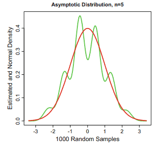
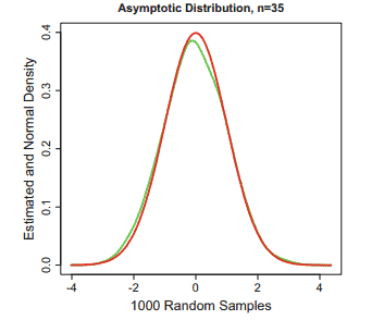
多元回归分析渐进(Multiple Regression Analysis Asymptotics)属于计量经济学领域,主要是一种数学上的统计分析方法,可以分析复杂情况下各影响因素的数学关系,在自然科学、社会和经济学等多个领域内应用广泛。
MATLAB代写
MATLAB 是一种用于技术计算的高性能语言。它将计算、可视化和编程集成在一个易于使用的环境中,其中问题和解决方案以熟悉的数学符号表示。典型用途包括:数学和计算算法开发建模、仿真和原型制作数据分析、探索和可视化科学和工程图形应用程序开发,包括图形用户界面构建MATLAB 是一个交互式系统,其基本数据元素是一个不需要维度的数组。这使您可以解决许多技术计算问题,尤其是那些具有矩阵和向量公式的问题,而只需用 C 或 Fortran 等标量非交互式语言编写程序所需的时间的一小部分。MATLAB 名称代表矩阵实验室。MATLAB 最初的编写目的是提供对由 LINPACK 和 EISPACK 项目开发的矩阵软件的轻松访问,这两个项目共同代表了矩阵计算软件的最新技术。MATLAB 经过多年的发展,得到了许多用户的投入。在大学环境中,它是数学、工程和科学入门和高级课程的标准教学工具。在工业领域,MATLAB 是高效研究、开发和分析的首选工具。MATLAB 具有一系列称为工具箱的特定于应用程序的解决方案。对于大多数 MATLAB 用户来说非常重要,工具箱允许您学习和应用专业技术。工具箱是 MATLAB 函数(M 文件)的综合集合,可扩展 MATLAB 环境以解决特定类别的问题。可用工具箱的领域包括信号处理、控制系统、神经网络、模糊逻辑、小波、仿真等。