如果你也在 怎样代写多元统计分析Multivariate Statistical Analysis这个学科遇到相关的难题,请随时右上角联系我们的24/7代写客服。
多变量统计分析被认为是评估地球化学异常与任何单独变量和变量之间相互影响的意义的有用工具。
statistics-lab™ 为您的留学生涯保驾护航 在代写多元统计分析Multivariate Statistical Analysis方面已经树立了自己的口碑, 保证靠谱, 高质且原创的统计Statistics代写服务。我们的专家在代写多元统计分析Multivariate Statistical Analysis代写方面经验极为丰富,各种代写多元统计分析Multivariate Statistical Analysis相关的作业也就用不着说。
我们提供的多元统计分析Multivariate Statistical Analysis及其相关学科的代写,服务范围广, 其中包括但不限于:
- Statistical Inference 统计推断
- Statistical Computing 统计计算
- Advanced Probability Theory 高等概率论
- Advanced Mathematical Statistics 高等数理统计学
- (Generalized) Linear Models 广义线性模型
- Statistical Machine Learning 统计机器学习
- Longitudinal Data Analysis 纵向数据分析
- Foundations of Data Science 数据科学基础
统计代写|多元统计分析代写Multivariate Statistical Analysis代考|The Principal Components
Let $\mathbf{x}=\left(x_{1}, x_{2}, \cdots, x_{p}\right)^{\mathrm{T}}$ be a set of $p$ continuous variables. The basic idea of a PCA method is to transform the set of variables $\left(x_{1}, x_{2}, \cdots, x_{p}\right)$ into a smaller set of uncorrelated new variables and try to explain most variability in the original variables $\mathbf{x}$ through these new variables. Specifically, let
$$
\mu=E(\mathbf{x})=\left(\mu_{1}, \mu_{2}, \cdots, \mu_{p}\right)^{\mathrm{T}}, \quad \Sigma=\operatorname{Cov}(\mathbf{x})=\left(\sigma_{i j}\right)_{p \times p}
$$
be the mean vector and the covariance matrix of $x$ respectively. Note that the mean vector $\boldsymbol{\mu}$ represents the center of $\mathbf{x}$, and the covariance matrix $\Sigma$ represents the vari-
ations (the diagonal elements of $\Sigma$ ) and correlations (the off-diagonal elements of $\Sigma$ ) of the random vector $\mathbf{x}$.
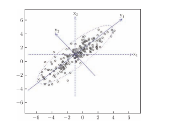
For ease interpretation, we usually replace $\mathbf{x}$ by its centered version $\mathbf{x}-\boldsymbol{\mu}$. We consider the following linear combinations of the components of vector $\mathrm{x}-\mu$
$$
\begin{array}{r}
y_{1}=\mathbf{a}{1}^{\mathrm{T}}(\mathbf{x}-\mu)=a{11}\left(x_{1}-\mu_{1}\right)+a_{12}\left(x_{2}-\mu_{2}\right)+\cdots+a_{1 p}\left(x_{p}-\mu_{p}\right), \
y_{2}=\mathbf{a}{2}^{\mathrm{T}}(\mathbf{x}-\mu)=a{21}\left(x_{1}-\mu_{1}\right)+a_{22}\left(x_{2}-\mu_{2}\right)+\cdots+a_{2 p}\left(x_{p}-\mu_{p}\right) \
\cdots \cdots \
y_{p}=\mathbf{a}{p}^{\mathrm{T}}(\mathbf{x}-\boldsymbol{\mu})=a{p 1}\left(x_{1}-\mu_{1}\right)+a_{p 2}\left(x_{2}-\mu_{2}\right)+\cdots+a_{p p}\left(x_{p}-\mu_{p}\right),
\end{array}
$$
where $\mathbf{a}{k}=\left(a{k 1}, a_{k 2}, \cdots, a_{k p}\right)^{\mathrm{T}}$ is a vector of constants. That is, each $y_{k}$ is a linear combination of the original random vector $x$. Then, we can show that
$$
\operatorname{Var}\left(y_{i}\right)=\mathbf{a}{i}^{\mathrm{T}} \Sigma \mathbf{a}{i}, \quad \operatorname{Cov}\left(y_{i}, y_{j}\right)=\mathbf{a}{i}^{\mathrm{T}} \Sigma \mathbf{a}{j}, \quad i, j=1,2, \cdots, p .
$$
Note that the variance of $y_{i}$ increases as the length of $\mathbf{a}{i}$, denoted by $\left|\mathbf{a}{i}\right|$, increases. To ensure uniqueness of $\mathbf{a}{i}$, we can assume that $\mathbf{a}{i}$ is a unit vector, i.e., $\left|\mathbf{a}{i}\right|=1$, for $i=1,2, \cdots, p$. This can be easily done since a vector can always be rescaled to have length of one. The first principal component (PC) is defined as $$ y{1}=\mathbf{a}{1}^{\top} \mathbf{x} $$ where $\mathbf{a}{1}$ is chosen to maximize the variance $\operatorname{Var}\left(\mathbf{a}{1}^{\mathrm{T}} \mathbf{x}\right)$ over all constant vectors $\mathbf{a}{1}$ subject to the restriction $\left|\mathbf{a}{1}\right|=1$. The second principal component (PC) is defined as $$ y{2}=\mathbf{a}{2}^{\mathbf{T}} \mathbf{x} $$ where $\mathbf{a}{2}$ is chosen to maximize the variance $\operatorname{Var}\left(\mathbf{a}{2}^{\mathrm{T}} \mathbf{x}\right)$ over all constant vectors $\mathbf{a}{2}$ subject to the restrictions
$$
\left|\mathbf{a}{2}\right|=1, \quad \operatorname{Cov}\left(\mathbf{a}{2}^{\mathrm{T}} \mathbf{x}, \mathbf{a}_{1}^{\mathrm{T}} \mathbf{x}\right)=0
$$
统计代写|多元统计分析代写Multivariate Statistical Analysis代考|Choose Number of Principal Components
The purpose of $\mathrm{PCA}$ is to reduce dimension, i.e., reduce the number of variables. In practice, we need to decide how many dimensions we can reduce without much loss of information. In other words, we should decide how many principal components should be retained. This question can be answered by the amount of variation that can be explained through the first few principal components.
Note that the total variation (variance) in the data is
$$
\operatorname{tr}(\Sigma)=\sigma_{11}+\cdots+\sigma_{p p}=\lambda_{1}+\cdots+\lambda_{p}
$$
Thus, the importance of the $\mathrm{j}$-th $\mathrm{PC}$ can be measured by the ratio
$$
\frac{\lambda_{j}}{t r(\Sigma)}, \quad j=1,2, \cdots, p
$$
i.e,, the proportion of the total variability explained by the $j$-th $\mathrm{PC}$. For example, the importance of the first two PCs can be measured by the ratio
$$
\frac{\lambda_{1}+\lambda_{2}}{\operatorname{tr}(\Sigma)}
$$
If the first few PCs can explain most (e.g., $70 \% \sim 80 \%$ ) of the total variability, then these first few PCs can replace all the original $p$ variables without much loss of information, where the information is measured by the variability. For example, if the first two $\mathrm{PCs}\left(y_{1}\right.$ and $\left.y_{2}\right)$ can explain $70 \%$ variation in the original $p=10$ variables $\left(x_{1}, \cdots, x_{10}\right)$, i.e., if $\left(\lambda_{1}+\lambda_{2}\right) / \operatorname{tr}(\Sigma)=0.7$, we can just use the two new variables (i.e., the first two PCs $y_{1}$ and $\left.y_{2}\right)$ instead of the original 10 variables $\left(x_{1}, \cdots, x_{10}\right)$ in data analysis, so the dimension of the data space is reduced from 10 to 2 (a big reduction in dimension!). Then, we can use graphical tools to display the “new data” on the two new variables. Although we loss some information by using the two new variables instead of the original ten variables, we gain a lot in data analysis, such as better parameter estimates and better use of graphical tools.
There have been some suggestions in the literature on choosing the number of principal components. For example, some authors suggest that, if we do PCA on the correlation matrix (not the covariance matrix), then the eigenvalues greater than 1 should be retained, which means that the PCs with variance larger than 1 are retained. A scree plot (see Figure 2.4) is also a useful visual aid for deciding the number of principal components. We will illustrate these methods in the $R$ examples later. These methods are rules of thumb and should be treated as a guideline only. In real applications, however, we do not need to follow these guidelines strictly. The decision for choosing the number of principal components should be based on subjectmatter interpretation, i.e., whether the chosen principal components make good sense in the particular problem under consideration and whether the chosen number of principal components can help us in data analysis. For example, if we choose two principal components, we will be able to use graphical tools, but if we choose three or more principal components, we are unable to use graphical tools. On the other hand, we usually hope that the chosen number of principal components can explain most of the variation in the data, such as at least $70 \%$ of the total variation. In summary, choosing the number of principal components should be guided by data analysis rather than certain strict rules.
统计代写|多元统计分析代写Multivariate Statistical Analysis代考|Considerations in Data Analysis
In practice, the true population mean vector $\mu$ and covariance matrix $\Sigma$ are unknown. Thus, in data analysis, we should use the sample estimates of the mean vector and the covariance matrix to replace the unknown population mean vector and covariance
matrix. Specifically, given a sample of data $\left{\mathbf{x}{1}, \cdots, \mathbf{x}{n}\right}$, where $\mathbf{x}{i}=\left(x{i 1}, \cdots, x_{i p}\right)^{\mathrm{T}}$, we can use the following sample mean vector $\overline{\mathbf{x}}=\hat{\mu}$ and sample covariance matrix $S=\hat{\Sigma}$ for PCA:
$$
\overline{\mathbf{x}}=\frac{1}{n} \sum_{i=1}^{n} \mathbf{x}{i}, \quad S=\left(\hat{\sigma}{i j}\right){p \times p}=\frac{1}{n-1} \sum{i=1}^{n}\left(\mathbf{x}{i}-\overline{\mathbf{x}}\right)\left(\mathbf{x}{i}-\overline{\mathbf{x}}\right)^{\mathrm{T}} .
$$
The accuracies of these estimates depend on the sample size $n$. The larger the sample size, the closer the sample estimates to the population parameters.
Note that PCA results may depend on the scales or units of the variables. For example, a distance $x_{1}$ can be measured in centermeter or in meter, and their values can differ by 100 times. The PCA results may depend on the scale (or unit) of $x_{1}$. Usually, it is desirable that all the variables in the original data have similar scales, i.e., the magnitudes of the values are comparable (e.g., not some values are around $0.0001$ while other values are around 10000 ). To address this issue, it is generally desirable to perform PCA on the correlation matrix $R$ rather than the original covariance matrix $\Sigma$, or perform PCA on the standardized data:
$$
z_{i j}=\frac{x_{i j}-\bar{x}{j}}{\sqrt{\sigma{j j}}}, \quad i=1,2, \cdots, n ; \quad k=1,2, \cdots, p,
$$
where $\bar{x}{j}=\sum{i=1}^{n} x_{i j} / n$, which are transformations of the original data, with mean 0 and variance $1 .$
Once we find the PCs, i.e., the new variables $y_{j}$ ‘s, we can convert the original data $x_{i j}$ into “new data” of the PCs $y_{j}$ ‘s. For example, for individual $i$, let
$$
\hat{y}{i k}=\hat{\mathbf{a}}{k}^{\mathrm{T}}\left(\mathbf{x}{i}-\overline{\mathbf{x}}\right), \quad i=1,2, \cdots, n ; \quad k=1,2, \cdots, p, $$ where $\hat{\mathbf{a}}{k}$ ‘s are the eigenvectors of the sample covariance matrix $\boldsymbol{S}=\hat{\Sigma}$ or the sample correlation matrix $\boldsymbol{R}$. These “new data”
$$
\left{\hat{y}{i k}: i=1,2, \cdots, n ; k=1,2, \cdots, p\right} $$ are called $P C$ scores, and they can be used for further analysis. For example, we may proceed with “new data” on the first two $\mathrm{PCs}\left{\hat{y}{i k}: i=1,2, \cdots, n ; k=1,2\right}$. in data analysis. In other words, data analysis is performed on the new data with two variables rather than the original data with $p$ variables.
Principal components are linear combinations of the original variables. Original variables have practical meanings, but the principal components do not always have practical meanings. However, sometimes we may be able to interpret interesting practical meanings for some principal components, as illustrated in Examples 2 and 3 in next section.
多元统计分析代考
统计代写|多元统计分析代写Multivariate Statistical Analysis代考|The Principal Components
让X=(X1,X2,⋯,Xp)吨成为一组p连续变量。PCA 方法的基本思想是变换变量集(X1,X2,⋯,Xp)成较小的一组不相关的新变量,并尝试解释原始变量中的大部分可变性X通过这些新变量。具体来说,让
μ=和(X)=(μ1,μ2,⋯,μp)吨,Σ=这(X)=(σ一世j)p×p
是平均向量和协方差矩阵X分别。注意平均向量μ代表中心X, 和协方差矩阵Σ代表变量
ations(的对角线元素Σ)和相关性(的非对角元素Σ) 的随机向量X.
为了便于解释,我们通常替换X以其居中的版本X−μ. 我们考虑向量分量的以下线性组合X−μ
是1=一个1吨(X−μ)=一个11(X1−μ1)+一个12(X2−μ2)+⋯+一个1p(Xp−μp), 是2=一个2吨(X−μ)=一个21(X1−μ1)+一个22(X2−μ2)+⋯+一个2p(Xp−μp) ⋯⋯ 是p=一个p吨(X−μ)=一个p1(X1−μ1)+一个p2(X2−μ2)+⋯+一个pp(Xp−μp),
在哪里一个ķ=(一个ķ1,一个ķ2,⋯,一个ķp)吨是一个常数向量。也就是说,每个是ķ是原始随机向量的线性组合X. 那么,我们可以证明
曾是(是一世)=一个一世吨Σ一个一世,这(是一世,是j)=一个一世吨Σ一个j,一世,j=1,2,⋯,p.
请注意,方差是一世随着长度的增加一个一世,表示为|一个一世|, 增加。为了保证唯一性一个一世, 我们可以假设一个一世是单位向量,即|一个一世|=1, 为了一世=1,2,⋯,p. 这可以很容易地完成,因为向量总是可以重新调整为长度为 1。第一主成分(PC)定义为
是1=一个1⊤X在哪里一个1选择最大化方差曾是(一个1吨X)在所有常数向量上一个1受限制|一个1|=1. 第二主成分(PC)定义为
是2=一个2吨X在哪里一个2选择最大化方差曾是(一个2吨X)在所有常数向量上一个2受限制
|一个2|=1,这(一个2吨X,一个1吨X)=0
统计代写|多元统计分析代写Multivariate Statistical Analysis代考|Choose Number of Principal Components
的目的磷C一个就是降维,即减少变量个数。在实践中,我们需要决定在不丢失太多信息的情况下可以减少多少维。换句话说,我们应该决定应该保留多少主成分。这个问题可以通过前几个主要成分可以解释的变化量来回答。
请注意,数据中的总变异(方差)为
tr(Σ)=σ11+⋯+σpp=λ1+⋯+λp
因此, 的重要性j-th磷C可以通过比例来衡量
λj吨r(Σ),j=1,2,⋯,p
即,由j-th磷C. 例如,前两台 PC 的重要性可以通过比率来衡量
λ1+λ2tr(Σ)
如果前几台 PC 可以解释最多(例如,70%∼80%) 的总可变性,那么这些前几台 PC 可以取代所有原来的p变量而不会丢失太多信息,其中信息是通过可变性来衡量的。例如,如果前两个磷Cs(是1和是2)可以解释70%原作的变化p=10变量(X1,⋯,X10),即,如果(λ1+λ2)/tr(Σ)=0.7,我们可以只使用两个新变量(即前两台 PC是1和是2)而不是原来的 10 个变量(X1,⋯,X10)在数据分析中,所以数据空间的维度从 10 降到了 2(降维大了!)。然后,我们可以使用图形工具来显示两个新变量上的“新数据”。虽然我们通过使用两个新变量而不是原来的十个变量丢失了一些信息,但我们在数据分析中获得了很多,例如更好的参数估计和更好地使用图形工具。
文献中有一些关于选择主成分数量的建议。例如,一些作者建议,如果我们对相关矩阵(而不是协方差矩阵)进行 PCA,那么应该保留大于 1 的特征值,这意味着保留方差大于 1 的 PC。碎石图(见图 2.4)也是确定主成分数量的有用视觉辅助工具。我们将在R后面的例子。这些方法是经验法则,应仅作为指导。然而,在实际应用中,我们不需要严格遵循这些准则。选择主成分数量的决定应基于主题解释,即选择的主成分是否对所考虑的特定问题有意义,以及选择的主成分数量是否可以帮助我们进行数据分析。例如,如果我们选择两个主成分,我们将能够使用图形工具,但如果我们选择三个或更多主成分,我们将无法使用图形工具。另一方面,我们通常希望所选择的主成分数量能够解释数据中的大部分变化,例如至少70%的总变异。总之,选择主成分的数量应该以数据分析为指导,而不是某些严格的规则。
统计代写|多元统计分析代写Multivariate Statistical Analysis代考|Considerations in Data Analysis
在实践中,真实总体平均向量μ和协方差矩阵Σ是未知的。因此,在数据分析中,我们应该使用均值向量和协方差矩阵的样本估计值来代替未知的总体均值向量和协方差
矩阵。具体来说,给定一个数据样本\left{\mathbf{x}{1}, \cdots, \mathbf{x}{n}\right}\left{\mathbf{x}{1}, \cdots, \mathbf{x}{n}\right}, 在哪里X一世=(X一世1,⋯,X一世p)吨,我们可以使用下面的样本均值向量X¯=μ^和样本协方差矩阵小号=Σ^对于 PCA:
X¯=1n∑一世=1nX一世,小号=(σ^一世j)p×p=1n−1∑一世=1n(X一世−X¯)(X一世−X¯)吨.
这些估计的准确性取决于样本量n. 样本量越大,样本估计值越接近总体参数。
请注意,PCA 结果可能取决于变量的尺度或单位。例如,距离X1可以用中心计或米来测量,它们的值可以相差100倍。PCA 结果可能取决于X1. 通常,希望原始数据中的所有变量都具有相似的尺度,即值的大小是可比较的(例如,不是某些值在0.0001而其他值在 10000 左右)。为了解决这个问题,通常需要对相关矩阵执行 PCAR而不是原来的协方差矩阵Σ,或对标准化数据执行 PCA:
和一世j=X一世j−X¯jσjj,一世=1,2,⋯,n;ķ=1,2,⋯,p,
在哪里X¯j=∑一世=1nX一世j/n,它们是原始数据的变换,均值为 0,方差为1.
一旦我们找到 PC,即新变量是j的,我们可以转换原始数据X一世j进入 PC 的“新数据”是j的。例如,对于个人一世, 让
是^一世ķ=一个^ķ吨(X一世−X¯),一世=1,2,⋯,n;ķ=1,2,⋯,p,在哪里一个^ķ是样本协方差矩阵的特征向量小号=Σ^或样本相关矩阵R. 这些“新数据”
\left{\hat{y}{i k}: i=1,2, \cdots, n ; k=1,2, \cdots, p\right}\left{\hat{y}{i k}: i=1,2, \cdots, n ; k=1,2, \cdots, p\right}被称为磷C分数,它们可用于进一步分析。例如,我们可以对前两个进行“新数据”\mathrm{PCs}\left{\hat{y}{i k}: i=1,2, \cdots, n ; k=1,2\右}\mathrm{PCs}\left{\hat{y}{i k}: i=1,2, \cdots, n ; k=1,2\右}. 在数据分析中。换句话说,数据分析是对具有两个变量的新数据而不是具有p变量。
主成分是原始变量的线性组合。原始变量具有实际意义,但主成分并不总是具有实际意义。但是,有时我们可能能够解释一些主成分的有趣的实际含义,如下一节的示例 2 和示例 3 所示。

统计代写请认准statistics-lab™. statistics-lab™为您的留学生涯保驾护航。
金融工程代写
金融工程是使用数学技术来解决金融问题。金融工程使用计算机科学、统计学、经济学和应用数学领域的工具和知识来解决当前的金融问题,以及设计新的和创新的金融产品。
非参数统计代写
非参数统计指的是一种统计方法,其中不假设数据来自于由少数参数决定的规定模型;这种模型的例子包括正态分布模型和线性回归模型。
广义线性模型代考
广义线性模型(GLM)归属统计学领域,是一种应用灵活的线性回归模型。该模型允许因变量的偏差分布有除了正态分布之外的其它分布。
术语 广义线性模型(GLM)通常是指给定连续和/或分类预测因素的连续响应变量的常规线性回归模型。它包括多元线性回归,以及方差分析和方差分析(仅含固定效应)。
有限元方法代写
有限元方法(FEM)是一种流行的方法,用于数值解决工程和数学建模中出现的微分方程。典型的问题领域包括结构分析、传热、流体流动、质量运输和电磁势等传统领域。
有限元是一种通用的数值方法,用于解决两个或三个空间变量的偏微分方程(即一些边界值问题)。为了解决一个问题,有限元将一个大系统细分为更小、更简单的部分,称为有限元。这是通过在空间维度上的特定空间离散化来实现的,它是通过构建对象的网格来实现的:用于求解的数值域,它有有限数量的点。边界值问题的有限元方法表述最终导致一个代数方程组。该方法在域上对未知函数进行逼近。[1] 然后将模拟这些有限元的简单方程组合成一个更大的方程系统,以模拟整个问题。然后,有限元通过变化微积分使相关的误差函数最小化来逼近一个解决方案。
tatistics-lab作为专业的留学生服务机构,多年来已为美国、英国、加拿大、澳洲等留学热门地的学生提供专业的学术服务,包括但不限于Essay代写,Assignment代写,Dissertation代写,Report代写,小组作业代写,Proposal代写,Paper代写,Presentation代写,计算机作业代写,论文修改和润色,网课代做,exam代考等等。写作范围涵盖高中,本科,研究生等海外留学全阶段,辐射金融,经济学,会计学,审计学,管理学等全球99%专业科目。写作团队既有专业英语母语作者,也有海外名校硕博留学生,每位写作老师都拥有过硬的语言能力,专业的学科背景和学术写作经验。我们承诺100%原创,100%专业,100%准时,100%满意。
随机分析代写
随机微积分是数学的一个分支,对随机过程进行操作。它允许为随机过程的积分定义一个关于随机过程的一致的积分理论。这个领域是由日本数学家伊藤清在第二次世界大战期间创建并开始的。
时间序列分析代写
随机过程,是依赖于参数的一组随机变量的全体,参数通常是时间。 随机变量是随机现象的数量表现,其时间序列是一组按照时间发生先后顺序进行排列的数据点序列。通常一组时间序列的时间间隔为一恒定值(如1秒,5分钟,12小时,7天,1年),因此时间序列可以作为离散时间数据进行分析处理。研究时间序列数据的意义在于现实中,往往需要研究某个事物其随时间发展变化的规律。这就需要通过研究该事物过去发展的历史记录,以得到其自身发展的规律。
回归分析代写
多元回归分析渐进(Multiple Regression Analysis Asymptotics)属于计量经济学领域,主要是一种数学上的统计分析方法,可以分析复杂情况下各影响因素的数学关系,在自然科学、社会和经济学等多个领域内应用广泛。
MATLAB代写
MATLAB 是一种用于技术计算的高性能语言。它将计算、可视化和编程集成在一个易于使用的环境中,其中问题和解决方案以熟悉的数学符号表示。典型用途包括:数学和计算算法开发建模、仿真和原型制作数据分析、探索和可视化科学和工程图形应用程序开发,包括图形用户界面构建MATLAB 是一个交互式系统,其基本数据元素是一个不需要维度的数组。这使您可以解决许多技术计算问题,尤其是那些具有矩阵和向量公式的问题,而只需用 C 或 Fortran 等标量非交互式语言编写程序所需的时间的一小部分。MATLAB 名称代表矩阵实验室。MATLAB 最初的编写目的是提供对由 LINPACK 和 EISPACK 项目开发的矩阵软件的轻松访问,这两个项目共同代表了矩阵计算软件的最新技术。MATLAB 经过多年的发展,得到了许多用户的投入。在大学环境中,它是数学、工程和科学入门和高级课程的标准教学工具。在工业领域,MATLAB 是高效研究、开发和分析的首选工具。MATLAB 具有一系列称为工具箱的特定于应用程序的解决方案。对于大多数 MATLAB 用户来说非常重要,工具箱允许您学习和应用专业技术。工具箱是 MATLAB 函数(M 文件)的综合集合,可扩展 MATLAB 环境以解决特定类别的问题。可用工具箱的领域包括信号处理、控制系统、神经网络、模糊逻辑、小波、仿真等。