如果你也在 怎样代写实验设计experimental design这个学科遇到相关的难题,请随时右上角联系我们的24/7代写客服。
实验设计是一个概念,用于有效地组织、进行和解释实验结果,确保通过进行少量的试验获得尽可能多的有用信息。
statistics-lab™ 为您的留学生涯保驾护航 在代写实验设计experimental designatistical Modelling方面已经树立了自己的口碑, 保证靠谱, 高质且原创的统计Statistics代写服务。我们的专家在代写实验设计experimental design代写方面经验极为丰富,各种代写实验设计experimental design相关的作业也就用不着说。
我们提供的实验设计experimental design及其相关学科的代写,服务范围广, 其中包括但不限于:
- Statistical Inference 统计推断
- Statistical Computing 统计计算
- Advanced Probability Theory 高等楖率论
- Advanced Mathematical Statistics 高等数理统计学
- (Generalized) Linear Models 广义线性模型
- Statistical Machine Learning 统计机器学习
- Longitudinal Data Analysis 纵向数据分析
- Foundations of Data Science 数据科学基础
统计代写|实验设计作业代写experimental design代考|TRANSFORMATIONS TO OBTAIN LINEARITY
Two variables, $x$ and $y$, may be closely related but the relationship may not be linear. Ideally, theoretical clues would be present wh1ch point to a particular relationship such as an exponential growth model which is common in blology. Without such clues, we could firstly examine a scatter plot of $y$ against $x$.
Sometimes we may recognize a mathematical model which $f$ its the data well. Otherwise, we try to choose a simple transformation such
as ralsing the variable to a power p as in Table 1.4.1. A power of 1 leaves the variable unchanged, that is as raw data. As we proceed up or down the table from 1 , the strength of the transformation increases; as we move up the table the transformation stretohes larger values relatively more than smaller ones. Although the exponential does not flt in very well, we nave included $1 t$ as $1 t 1 s$ the inverse of the logarithmic transformation. other fractional powers oould be used but they may be difficult to interpret.
It would be feasible to transform either $y$ or $x$, and, indeed, a transformation of $y$ would be equivalent to the inverse transformation of $x$. For example, squaring $y$ would be equivalent to taking the square root of $x$. If there are two or more predictor variables, it is often advisable to transform these in different ways nather than $y$, for if y is transformed to be linearly related to one predictor variable it may then not be 1 inear ly related to another.
In Eigure 1.4.1, it is clear that we should stretoh out the graph by increasing large $x$ values, or, alternatively; reduce large $y$ values. Thus, we could try changing $x$ to $x$-squared, or $y$ to the square root of $y_{*}$ One point to be kept in mind here is that for p>0, $y=0$ when $x=0$ so that it may be advisable before invoking the power transformation to change the origin; in partfoular, we could onange y to $(y-a)$, and a good guess may be a $=30$. In Figure $1.4 .2$, it seems that large $x$ values and large $y$ values should be reduced suggesting that a reciprooal transformation may be appropriate. This would require the $x$ and $y$ axes to be asymptotes which, in particular, would
mean that a constant, perhaps 14 , should be subtracted from $y$. We could try changing
$$
\begin{aligned}
&y \text { to }(y-14)^{-1} \
&\text { or } y \text { to }(y=14)^{-0.5} \
&\text { or } x \text { to } x{ }^{-1} \
&\text { or } x \text { to } x=0.5
\end{aligned}
$$
统计代写|实验设计作业代写experimental design代考|FITTING A MODEL USING VECTORS AND MATRICES
Appendix A contains a review of vectors, vector spaces and matrices and some readers may wish to refer to that section while reading the following.
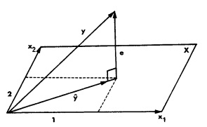
In regression, we consider the relationship between a string of values of the dependent variable, $y$, and one or more strings of corresponding values of the predictor variables, the $x$ ‘s. It is useful to think of each string as a vector for it turns out that the relationships of interest between the variables are encapsulated in the lengths of the vectors and the angles between them. For the simple Example $1.3 .1$, the $x$ and $y$ readings can be written as column vectors:
The simplest model for this example would be a line through the origin
$$
\mathrm{y}{\mathrm{i}}=B \mathrm{X}{\mathrm{i}}+\mathrm{E}{i} $$ or $\mathbf{y}=\beta \mathbf{x}+\boldsymbol{\varepsilon}$ in vector terms The normal equation $1 \mathrm{~s}$ $b \sum x{1}^{2}=\sum x_{1}^{y_{1}}$
or $\left(x^{T} x\right) b=x^{T} y$
giving $b=\left(x^{T} \mathbf{y}\right) /\left(x^{T} \mathbf{x}\right)=0.973$
$(1.5 .2)$
For each value of $x$ we can calculate the predicted value of $y$ as
$$
\mathbf{y}=b x \text { or } x b=\left|\begin{array}{l}
0.5 \
1.0 \
1.5 \
2.0 \
2.5
\end{array}\right| 0.973=\left|\begin{array}{l}
0.486 \
0.973 \
1.459 \
1.945 \
2.432
\end{array}\right|
$$
The predicted value can also be written as
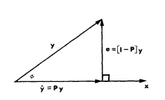
$$
y=x b=x\left(x^{T} x\right)^{-1} x^{T} y=P y
$$
The matrix $P=x\left(x^{T} \mathbf{x}\right)^{-1} x^{T}$ is termed the projection matrix. More is said about this in section 1.7. Notice that for this case with $n=5$, $P$ is a $5 \times 5$ matrix, namely.
统计代写|实验设计作业代写experimental design代考|DEVIATIONS FROM MEANS
It is common practice when fitting a model to use the original (also called raw) data and to include $1 n$ the model a $y=i n t e r c e p t ~ t e r m ~(a l s o ~$ called a constant, or general mean). Most computer programs would convert the raw data to deviations from the mean, as these are used in such statistics as the correlation coefficient. Converting to deviations has the advantage of removing a parameter from the model, making 1 t easier to man1 pulate. Sometimes an examination of the deviations shows up trends which are not as clearly noticeable in the raw data. Problem $2.1$ is an example where deviations from the mean prove useful. It turns out that the estimated coefficients will be the same for the raw data with constant term as with the data 1 n deviation form.
For this section we change our notation slightly to make 1 t clear whether we are referring to the raw data (which we indicate by capital letters, $X, Y$, etc) or deviations from means (lower case $x$, $y$, etc).
$1.6 .1$ Estimates
Ignoring subsor ipts for simplicity, we can write for the case of one predictor variable,
$$
x=X=\bar{X} \text { and } y=Y-\bar{Y}
$$
where $\vec{X}$ and $\vec{Y}$ are the sample means. For the model
$$
\mathrm{y}=8 x+\varepsilon
$$
we saw in $(1.2 .7)$ the least squares estimates are given by
$\begin{aligned} b &=\sum_{1}^{y_{1} / 2 x_{1}^{2}} \quad(\text { from } 1.2 .7) \ &=\mathrm{S}{x y} / \mathrm{S}{x x} \end{aligned} \quad$ (def ined by 1.2.13)
$(1.6 .2)$
Notice that the predicted value of $y$ in this case is $\hat{y}=b x$
实验设计代考
统计代写|实验设计作业代写experimental design代考|TRANSFORMATIONS TO OBTAIN LINEARITY
两个变量,X和是的, 可能密切相关,但关系可能不是线性的。理想情况下,理论线索将指向特定关系,例如在 bloology 中常见的指数增长模型。如果没有这些线索,我们可以先检查一个散点图是的反对X.
有时我们可能会认识到一个数学模型F它的数据很好。否则,我们尝试选择一个简单的转换,例如
如表 1.4.1 所示,将变量转换为幂 p。1 的幂保持变量不变,即作为原始数据。当我们从 1 开始向上或向下移动时,转换的强度会增加;当我们在表格中向上移动时,转换比较小的值相对更多地延伸较大的值。虽然指数并没有很好地适应,但我们没有包括1吨作为1吨1s对数变换的倒数。可以使用其他分数幂,但它们可能难以解释。
改造任何一个都是可行的是的或者X,而且,事实上,一个转变是的将相当于的逆变换X. 例如,平方是的相当于取平方根X. 如果有两个或多个预测变量,通常建议以不同的方式转换它们,而不是是的,因为如果 y 被转换为与一个预测变量线性相关,则它可能与另一个变量不是 1 密切相关。
在 Eigure 1.4.1 中,很明显我们应该通过增加X价值观,或者,或者,减少大是的价值观。因此,我们可以尝试改变X到X-平方,或是的的平方根是的∗这里要记住的一点是,对于 p>0,是的=0什么时候X=0以便在调用功率转换以更改原点之前可能是可取的;在partfoular,我们可以onange y to(是的−一种), 一个好的猜测可能是=30. 如图1.4.2, 好像很大X值和大是的值应该减少,这表明互惠变换可能是合适的。这将需要X和是的轴是渐近线,尤其是
意味着应该减去一个常数,也许是 14是的. 我们可以尝试改变
是的 到 (是的−14)−1 或者 是的 到 (是的=14)−0.5 或者 X 到 X−1 或者 X 到 X=0.5
统计代写|实验设计作业代写experimental design代考|FITTING A MODEL USING VECTORS AND MATRICES
附录 A 包含对向量、向量空间和矩阵的回顾,一些读者可能希望在阅读以下内容时参考该部分。
在回归中,我们考虑因变量的一串值之间的关系,是的,以及一串或多串对应的预测变量值,X的。将每个字符串视为一个向量是很有用的,因为事实证明,变量之间感兴趣的关系被封装在向量的长度和它们之间的角度中。对于简单的示例1.3.1, 这X和是的读数可以写成列向量:
这个例子最简单的模型是一条穿过原点的线
是的一世=乙X一世+和一世或者是的=bX+e用向量表示 正规方程1 s b∑X12=∑X1是的1
或者(X吨X)b=X吨是的
给予b=(X吨是的)/(X吨X)=0.973
(1.5.2)
对于每个值X我们可以计算出预测值是的作为
是的=bX 或者 Xb=|0.5 1.0 1.5 2.0 2.5|0.973=|0.486 0.973 1.459 1.945 2.432|
预测值也可以写成
是的=Xb=X(X吨X)−1X吨是的=磷是的
矩阵磷=X(X吨X)−1X吨称为投影矩阵。1.7 节对此进行了更多说明。请注意,对于这种情况n=5, 磷是一个5×5矩阵,即。
统计代写|实验设计作业代写experimental design代考|DEVIATIONS FROM MEANS
拟合模型以使用原始(也称为原始)数据并包含1n模型是的=一世n吨和rC和p吨 吨和r米 (一种ls这 称为常数或一般平均值)。大多数计算机程序会将原始数据转换为与平均值的偏差,因为这些数据用于相关系数等统计数据中。转换为偏差具有从模型中删除参数的优点,使 1 t 更容易计算。有时,对偏差的检查会发现在原始数据中不那么明显的趋势。问题2.1是一个证明偏离均值有用的例子。事实证明,具有常数项的原始数据的估计系数与数据 1 n 偏差形式的估计系数相同。
对于本节,我们稍微改变我们的符号,以明确我们是否指的是原始数据(我们用大写字母表示,X,是的等)或偏离均值(小写X, 是的, ETC)。
1.6.1估计
为简单起见忽略 subsor ipts,我们可以写一个预测变量的情况,
X=X=X¯ 和 是的=是的−是的¯
在哪里X→和是的→是样本均值。对于模型
是的=8X+e
我们在(1.2.7)最小二乘估计由下式给出
b=∑1是的1/2X12( 从 1.2.7) =小号X是的/小号XX(由 1.2.13 定义)
(1.6.2)
注意预测值是的在这种情况下是是的^=bX

统计代写请认准statistics-lab™. statistics-lab™为您的留学生涯保驾护航。
金融工程代写
金融工程是使用数学技术来解决金融问题。金融工程使用计算机科学、统计学、经济学和应用数学领域的工具和知识来解决当前的金融问题,以及设计新的和创新的金融产品。
非参数统计代写
非参数统计指的是一种统计方法,其中不假设数据来自于由少数参数决定的规定模型;这种模型的例子包括正态分布模型和线性回归模型。
广义线性模型代考
广义线性模型(GLM)归属统计学领域,是一种应用灵活的线性回归模型。该模型允许因变量的偏差分布有除了正态分布之外的其它分布。
术语 广义线性模型(GLM)通常是指给定连续和/或分类预测因素的连续响应变量的常规线性回归模型。它包括多元线性回归,以及方差分析和方差分析(仅含固定效应)。
有限元方法代写
有限元方法(FEM)是一种流行的方法,用于数值解决工程和数学建模中出现的微分方程。典型的问题领域包括结构分析、传热、流体流动、质量运输和电磁势等传统领域。
有限元是一种通用的数值方法,用于解决两个或三个空间变量的偏微分方程(即一些边界值问题)。为了解决一个问题,有限元将一个大系统细分为更小、更简单的部分,称为有限元。这是通过在空间维度上的特定空间离散化来实现的,它是通过构建对象的网格来实现的:用于求解的数值域,它有有限数量的点。边界值问题的有限元方法表述最终导致一个代数方程组。该方法在域上对未知函数进行逼近。[1] 然后将模拟这些有限元的简单方程组合成一个更大的方程系统,以模拟整个问题。然后,有限元通过变化微积分使相关的误差函数最小化来逼近一个解决方案。
tatistics-lab作为专业的留学生服务机构,多年来已为美国、英国、加拿大、澳洲等留学热门地的学生提供专业的学术服务,包括但不限于Essay代写,Assignment代写,Dissertation代写,Report代写,小组作业代写,Proposal代写,Paper代写,Presentation代写,计算机作业代写,论文修改和润色,网课代做,exam代考等等。写作范围涵盖高中,本科,研究生等海外留学全阶段,辐射金融,经济学,会计学,审计学,管理学等全球99%专业科目。写作团队既有专业英语母语作者,也有海外名校硕博留学生,每位写作老师都拥有过硬的语言能力,专业的学科背景和学术写作经验。我们承诺100%原创,100%专业,100%准时,100%满意。
随机分析代写
随机微积分是数学的一个分支,对随机过程进行操作。它允许为随机过程的积分定义一个关于随机过程的一致的积分理论。这个领域是由日本数学家伊藤清在第二次世界大战期间创建并开始的。
时间序列分析代写
随机过程,是依赖于参数的一组随机变量的全体,参数通常是时间。 随机变量是随机现象的数量表现,其时间序列是一组按照时间发生先后顺序进行排列的数据点序列。通常一组时间序列的时间间隔为一恒定值(如1秒,5分钟,12小时,7天,1年),因此时间序列可以作为离散时间数据进行分析处理。研究时间序列数据的意义在于现实中,往往需要研究某个事物其随时间发展变化的规律。这就需要通过研究该事物过去发展的历史记录,以得到其自身发展的规律。
回归分析代写
多元回归分析渐进(Multiple Regression Analysis Asymptotics)属于计量经济学领域,主要是一种数学上的统计分析方法,可以分析复杂情况下各影响因素的数学关系,在自然科学、社会和经济学等多个领域内应用广泛。
MATLAB代写
MATLAB 是一种用于技术计算的高性能语言。它将计算、可视化和编程集成在一个易于使用的环境中,其中问题和解决方案以熟悉的数学符号表示。典型用途包括:数学和计算算法开发建模、仿真和原型制作数据分析、探索和可视化科学和工程图形应用程序开发,包括图形用户界面构建MATLAB 是一个交互式系统,其基本数据元素是一个不需要维度的数组。这使您可以解决许多技术计算问题,尤其是那些具有矩阵和向量公式的问题,而只需用 C 或 Fortran 等标量非交互式语言编写程序所需的时间的一小部分。MATLAB 名称代表矩阵实验室。MATLAB 最初的编写目的是提供对由 LINPACK 和 EISPACK 项目开发的矩阵软件的轻松访问,这两个项目共同代表了矩阵计算软件的最新技术。MATLAB 经过多年的发展,得到了许多用户的投入。在大学环境中,它是数学、工程和科学入门和高级课程的标准教学工具。在工业领域,MATLAB 是高效研究、开发和分析的首选工具。MATLAB 具有一系列称为工具箱的特定于应用程序的解决方案。对于大多数 MATLAB 用户来说非常重要,工具箱允许您学习和应用专业技术。工具箱是 MATLAB 函数(M 文件)的综合集合,可扩展 MATLAB 环境以解决特定类别的问题。可用工具箱的领域包括信号处理、控制系统、神经网络、模糊逻辑、小波、仿真等。