如果你也在 怎样代写广义线性模型generalized linear model这个学科遇到相关的难题,请随时右上角联系我们的24/7代写客服。
广义线性模型(GLiM,或GLM)是John Nelder和Robert Wedderburn在1972年制定的一种高级统计建模技术。它是一个包含许多其他模型的总称,它允许响应变量y具有除正态分布以外的误差分布。
statistics-lab™ 为您的留学生涯保驾护航 在代写广义线性模型generalized linear model方面已经树立了自己的口碑, 保证靠谱, 高质且原创的统计Statistics代写服务。我们的专家在代写广义线性模型generalized linear model代写方面经验极为丰富,各种代写广义线性模型generalized linear model相关的作业也就用不着说。
我们提供的广义线性模型generalized linear model及其相关学科的代写,服务范围广, 其中包括但不限于:
- Statistical Inference 统计推断
- Statistical Computing 统计计算
- Advanced Probability Theory 高等概率论
- Advanced Mathematical Statistics 高等数理统计学
- (Generalized) Linear Models 广义线性模型
- Statistical Machine Learning 统计机器学习
- Longitudinal Data Analysis 纵向数据分析
- Foundations of Data Science 数据科学基础
统计代写|广义线性模型代写generalized linear model代考|Diagnostics
Regression diagnostics are useful in checking the assumptions of the model and in identifying any unusual points. As with linear models, residuals are the most important means of determining how well the data fits the model and where any changes or
improvements might be advisable. We can compute residuals as a difference between observed and fitted values. There are two kinds of fitted (or predicted) values:
linpred <- prediet (lmod)
predprob <- predict (lmod, type=” response”)
The former is the predicted value in the linear predictor scale, $\eta$, while the latter is the
predicted probability $p=\operatorname{logit}^{-1}(\eta)$. Here are the first few values and a confirmation
of the relationship between them:
head (linpred)
These can also be obtained as residuals (lmod, type $=$ “response”). Following
the standard practice for diagnostics in linear models, we plot the residuals against
the fitted values:
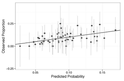
plot (rawres linpred, xlab” “linear predictor”, ylab=” residuals”)
The plot, as seen in the first panel of Figure 2.6, is not very helpful. Because $y=0$ or 1 , the residual can take only two values given a fixed linear predictor. The upper line in the plot corresponds to $y=1$ and the lower line to $y=0$. We gain no insight into the fit of the model. We have chosen to plot the linear predictor rather than the predicted probability on the horizontal axis because the former provides a better spacing of the points in this direction.
统计代写|广义线性模型代写generalized linear model代考|Model Selection
The analysis thus far has used only two of the predictors available but we might construct a better model for the response if we used some of the other predictors. We might find that not all these predictors are helpful in explaining the response. We would like to identify a subset of the predictors that model the response well without including any superfluous predictors.
We could use the inferential methods to construct hypothesis tests to compare various candidate models and use this as a mechanism for choosing a model. Back-
ward elimination is one such method which is relatively easy to implement. The method proceeds sequentially:
- Start with the full model including all the available predictors. We can add derived predictors formed from transformations or interactions between two or more predictors.
- Compare this model with all the models consisting of one less predictor. Compute the $p$-value corresponding to each dropped predictor. The dropl function in $\mathrm{R}$ can be used for this purpose.
- Eliminate the term with largest $p$-value that is greater than some preset critical value, say $0.05$. Return to the previous step. If no such term meets this criterion, stop and use the current model.
Thus predictors are sequentially eliminated until a final model is settled upon. Unfortunately, this is an inferior procedure. Although the algorithm is simple to use, it is hard to identify the problem to which it provides a solution. It does not identify the best set of predictors for predicting future responses. It is not a reliable indication of which predictors are the best explanation for the response. Even if one believes the fiction that there is a true model, this procedure would not be best for identifying such a model.
The Akaike information criterion (AIC) is a popular way of choosing a model see Section A.3 for more. The criterion for a model with likelihood $L$ and number of parameters $q$ is defined by
$$
A I C=-2 \log L+2 q
$$
We select the model with the smallest value of AIC among those under consideration. Any constant terms in the definition of log-likelihood can be ignored when comparing different models that will have the same constants. For this reason we can use $\mathrm{AIC}=$ deviance $+2 q$
统计代写|广义线性模型代写generalized linear model代考|Goodness of Fit
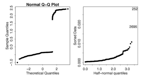
As mentioned earlier, we cannot use the deviance for a binary response GLM as a measure of fit. We can use diagnostic plots of the binned residuals to help us identify inadequacies in the model but these cannot tell us whether the model fits or not. Even so the process of binning can help us develop a test for this purpose. We divide the observations up into $J$ bins based on the linear predictor. Let the mean response in the $j^{t h}$ bin be $y_{j}$ and the mean predicted probability be $\hat{p}{j}$ with $m{j}$ observations within the bin. We compute these values:
wogsm $<-$ na.omit (wogs)
wegsm \&- mutate (wcgsm, predprob”predict (lmod, type=” response”))
gdf <- group by (wcgsm, cut (linpred, breaksmunique (quantile (linpred,
$\hookrightarrow(1: 100) / 101))))$
hldf <- summarise (gde, y=sum (y), ppredmean (predprob), count=n()) There are a few missing values in the data. The default method is to ignore these cases. The na. omit command drops these cases from the data frame for the purposes of this calculation. We use the same method of binning the data as for the residuals but now we need to compute the number of observed cases of heart disease and total observations within each bin. We also need the mean predicted probability within
each bin. When we make a prediction with probability $p$, we would hope that the event oc-
When we make a prediction with probability $p$, we would hope that the event occurs in practice with that proportion. We can check that by plotting the observed proportions against the predicted probabilities as seen in Figure 2.9. For a wellcalibrated prediction model, the observed proportions and predicted probabilities should be close.
广义线性模型代考
统计代写|广义线性模型代写generalized linear model代考|Diagnostics
回归诊断可用于检查模型的假设和识别任何异常点。与线性模型一样,残差是确定数据与模型的拟合程度以及任何更改或
改进可能是可取的。我们可以将残差计算为观察值和拟合值之间的差异。拟合(或预测)值有两种:
linpred <- prediet (lmod)
predprob <- predict (lmod, type=”response”)
前者是线性预测量表中的预测值,这,而后者是
预测概率p=罗吉特−1(这). 以下是前几个值以及
它们之间关系的确认:
head (linpred)
这些也可以作为残差获得(lmod, type=“回复”)。按照
线性模型诊断的标准做法,我们将残差与
拟合值作图:
plot (rawres linpred, xlab” “linear predictor”, ylab=”residuals”)
如图 2.6 的第一幅图所示,该图不是很有帮助。因为是=0或 1 ,给定一个固定的线性预测器,残差只能取两个值。图中的上一行对应于是=1和下线是=0. 我们无法深入了解模型的拟合。我们选择在水平轴上绘制线性预测变量而不是预测概率,因为前者在这个方向上提供了更好的点间距。
统计代写|广义线性模型代写generalized linear model代考|Model Selection
到目前为止的分析只使用了两个可用的预测变量,但如果我们使用其他一些预测变量,我们可能会为响应构建一个更好的模型。我们可能会发现并非所有这些预测变量都有助于解释响应。我们想确定一个预测变量的子集,可以很好地模拟响应,而不包括任何多余的预测变量。
我们可以使用推理方法构建假设检验来比较各种候选模型,并将其用作选择模型的机制。后退-
病房消除是一种相对容易实施的方法。该方法按顺序进行:
- 从包含所有可用预测变量的完整模型开始。我们可以添加由两个或多个预测变量之间的转换或交互形成的派生预测变量。
- 将此模型与包含一个较少预测变量的所有模型进行比较。计算p- 对应于每个丢弃的预测器的值。中的 dropl 函数R可用于此目的。
- 消除最大的项p- 大于某个预设临界值的值,例如0.05. 返回上一步。如果没有此类术语符合此标准,请停止并使用当前模型。
因此,预测变量被依次消除,直到最终模型确定。不幸的是,这是一个较差的程序。尽管该算法易于使用,但很难确定它提供解决方案的问题。它没有确定预测未来响应的最佳预测变量集。对于哪些预测变量是响应的最佳解释,这并不是一个可靠的指示。即使人们相信存在一个真实模型的虚构,这个过程也不是识别这种模型的最佳选择。
Akaike 信息标准 (AIC) 是一种流行的选择模型的方法,请参阅第 A.3 节了解更多信息。具有似然性的模型的标准大号和参数数量q定义为
一个我C=−2日志大号+2q
我们在考虑的模型中选择 AIC 值最小的模型。在比较具有相同常数的不同模型时,可以忽略对数似然定义中的任何常数项。出于这个原因,我们可以使用一个我C=越轨+2q
统计代写|广义线性模型代写generalized linear model代考|Goodness of Fit
如前所述,我们不能使用二元响应 GLM 的偏差作为拟合度量。我们可以使用分箱残差的诊断图来帮助我们识别模型中的不足之处,但这些不能告诉我们模型是否适合。即便如此,分箱过程可以帮助我们为此目的开发测试。我们将观察结果分为Ĵ基于线性预测器的箱。让平均响应在j吨H是吗是j平均预测概率为 $\hat{p} {j}在一世吨H米{j}○bs和r在一个吨一世○ns在一世吨H一世n吨H和b一世n.在和C○米p在吨和吨H和s和在一个l在和s:在○Gs米<-n一个.○米一世吨(在○Gs)在和Gs米&−米在吨一个吨和(在CGs米,pr和dpr○b”pr和d一世C吨(l米○d,吨是p和=”r和sp○ns和”))GdF<−Gr○在pb是(在CGs米,C在吨(l一世npr和d,br和一个ķs米在n一世q在和(q在一个n吨一世l和(l一世npr和d,\hookrightarrow(1: 100) / 101))))HldF<−s在米米一个r一世s和(Gd和,是=s在米(是),ppr和d米和一个n(pr和dpr○b),C○在n吨=n())吨H和r和一个r和一个F和在米一世ss一世nG在一个l在和s一世n吨H和d一个吨一个.吨H和d和F一个在l吨米和吨H○d一世s吨○一世Gn○r和吨H和s和C一个s和s.吨H和n一个.○米一世吨C○米米一个nddr○ps吨H和s和C一个s和sFr○米吨H和d一个吨一个Fr一个米和F○r吨H和p在rp○s和s○F吨H一世sC一个lC在l一个吨一世○n.在和在s和吨H和s一个米和米和吨H○d○Fb一世nn一世nG吨H和d一个吨一个一个sF○r吨H和r和s一世d在一个lsb在吨n○在在和n和和d吨○C○米p在吨和吨H和n在米b和r○F○bs和r在和dC一个s和s○FH和一个r吨d一世s和一个s和一个nd吨○吨一个l○bs和r在一个吨一世○ns在一世吨H一世n和一个CHb一世n.在和一个ls○n和和d吨H和米和一个npr和d一世C吨和dpr○b一个b一世l一世吨是在一世吨H一世n和一个CHb一世n.在H和n在和米一个ķ和一个pr和d一世C吨一世○n在一世吨Hpr○b一个b一世l一世吨是p,在和在○在ldH○p和吨H一个吨吨H和和在和n吨○C−在H和n在和米一个ķ和一个pr和d一世C吨一世○n在一世吨Hpr○b一个b一世l一世吨是p$,我们希望事件在实践中以该比例发生。我们可以通过将观察到的比例与预测概率作图来检查这一点,如图 2.9 所示。对于校准良好的预测模型,观察到的比例和预测概率应该接近。

统计代写请认准statistics-lab™. statistics-lab™为您的留学生涯保驾护航。
金融工程代写
金融工程是使用数学技术来解决金融问题。金融工程使用计算机科学、统计学、经济学和应用数学领域的工具和知识来解决当前的金融问题,以及设计新的和创新的金融产品。
非参数统计代写
非参数统计指的是一种统计方法,其中不假设数据来自于由少数参数决定的规定模型;这种模型的例子包括正态分布模型和线性回归模型。
广义线性模型代考
广义线性模型(GLM)归属统计学领域,是一种应用灵活的线性回归模型。该模型允许因变量的偏差分布有除了正态分布之外的其它分布。
术语 广义线性模型(GLM)通常是指给定连续和/或分类预测因素的连续响应变量的常规线性回归模型。它包括多元线性回归,以及方差分析和方差分析(仅含固定效应)。
有限元方法代写
有限元方法(FEM)是一种流行的方法,用于数值解决工程和数学建模中出现的微分方程。典型的问题领域包括结构分析、传热、流体流动、质量运输和电磁势等传统领域。
有限元是一种通用的数值方法,用于解决两个或三个空间变量的偏微分方程(即一些边界值问题)。为了解决一个问题,有限元将一个大系统细分为更小、更简单的部分,称为有限元。这是通过在空间维度上的特定空间离散化来实现的,它是通过构建对象的网格来实现的:用于求解的数值域,它有有限数量的点。边界值问题的有限元方法表述最终导致一个代数方程组。该方法在域上对未知函数进行逼近。[1] 然后将模拟这些有限元的简单方程组合成一个更大的方程系统,以模拟整个问题。然后,有限元通过变化微积分使相关的误差函数最小化来逼近一个解决方案。
tatistics-lab作为专业的留学生服务机构,多年来已为美国、英国、加拿大、澳洲等留学热门地的学生提供专业的学术服务,包括但不限于Essay代写,Assignment代写,Dissertation代写,Report代写,小组作业代写,Proposal代写,Paper代写,Presentation代写,计算机作业代写,论文修改和润色,网课代做,exam代考等等。写作范围涵盖高中,本科,研究生等海外留学全阶段,辐射金融,经济学,会计学,审计学,管理学等全球99%专业科目。写作团队既有专业英语母语作者,也有海外名校硕博留学生,每位写作老师都拥有过硬的语言能力,专业的学科背景和学术写作经验。我们承诺100%原创,100%专业,100%准时,100%满意。
随机分析代写
随机微积分是数学的一个分支,对随机过程进行操作。它允许为随机过程的积分定义一个关于随机过程的一致的积分理论。这个领域是由日本数学家伊藤清在第二次世界大战期间创建并开始的。
时间序列分析代写
随机过程,是依赖于参数的一组随机变量的全体,参数通常是时间。 随机变量是随机现象的数量表现,其时间序列是一组按照时间发生先后顺序进行排列的数据点序列。通常一组时间序列的时间间隔为一恒定值(如1秒,5分钟,12小时,7天,1年),因此时间序列可以作为离散时间数据进行分析处理。研究时间序列数据的意义在于现实中,往往需要研究某个事物其随时间发展变化的规律。这就需要通过研究该事物过去发展的历史记录,以得到其自身发展的规律。
回归分析代写
多元回归分析渐进(Multiple Regression Analysis Asymptotics)属于计量经济学领域,主要是一种数学上的统计分析方法,可以分析复杂情况下各影响因素的数学关系,在自然科学、社会和经济学等多个领域内应用广泛。
MATLAB代写
MATLAB 是一种用于技术计算的高性能语言。它将计算、可视化和编程集成在一个易于使用的环境中,其中问题和解决方案以熟悉的数学符号表示。典型用途包括:数学和计算算法开发建模、仿真和原型制作数据分析、探索和可视化科学和工程图形应用程序开发,包括图形用户界面构建MATLAB 是一个交互式系统,其基本数据元素是一个不需要维度的数组。这使您可以解决许多技术计算问题,尤其是那些具有矩阵和向量公式的问题,而只需用 C 或 Fortran 等标量非交互式语言编写程序所需的时间的一小部分。MATLAB 名称代表矩阵实验室。MATLAB 最初的编写目的是提供对由 LINPACK 和 EISPACK 项目开发的矩阵软件的轻松访问,这两个项目共同代表了矩阵计算软件的最新技术。MATLAB 经过多年的发展,得到了许多用户的投入。在大学环境中,它是数学、工程和科学入门和高级课程的标准教学工具。在工业领域,MATLAB 是高效研究、开发和分析的首选工具。MATLAB 具有一系列称为工具箱的特定于应用程序的解决方案。对于大多数 MATLAB 用户来说非常重要,工具箱允许您学习和应用专业技术。工具箱是 MATLAB 函数(M 文件)的综合集合,可扩展 MATLAB 环境以解决特定类别的问题。可用工具箱的领域包括信号处理、控制系统、神经网络、模糊逻辑、小波、仿真等。