如果你也在 怎样代写广义线性模型generalized linear model这个学科遇到相关的难题,请随时右上角联系我们的24/7代写客服。
广义线性模型(GLiM,或GLM)是John Nelder和Robert Wedderburn在1972年制定的一种高级统计建模技术。它是一个包含许多其他模型的总称,它允许响应变量y具有除正态分布以外的误差分布。
statistics-lab™ 为您的留学生涯保驾护航 在代写广义线性模型generalized linear model方面已经树立了自己的口碑, 保证靠谱, 高质且原创的统计Statistics代写服务。我们的专家在代写广义线性模型generalized linear model代写方面经验极为丰富,各种代写广义线性模型generalized linear model相关的作业也就用不着说。
我们提供的广义线性模型generalized linear model及其相关学科的代写,服务范围广, 其中包括但不限于:
- Statistical Inference 统计推断
- Statistical Computing 统计计算
- Advanced Probability Theory 高等概率论
- Advanced Mathematical Statistics 高等数理统计学
- (Generalized) Linear Models 广义线性模型
- Statistical Machine Learning 统计机器学习
- Longitudinal Data Analysis 纵向数据分析
- Foundations of Data Science 数据科学基础
统计代写|广义线性模型代写generalized linear model代考|Estimation Problems
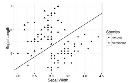
Estimation of the logistic regression model using the Fisher scoring algorithm, described in Section 8.2, is usually fast. However, difficulties can sometimes arise. When convergence fails, it is sometimes due to a problem exhibited by the following dataset. We take a subset of the famous Fisher Iris data to consider only two of the three species of Iris and use only two of the potential predictors:
ibrary (dplyr)
irisr <- filter(iris, Species ! “virginica”) to ? select (Sepal. Width,
$\rightarrow$ Sepal. Length, Species)
We plot the data using a different shape of plotting symbol for the two species:
(p <- ggplot(irisr, aes (x=Sepa1. Width, y=Sepal. Length, shape=Species))
$\hookrightarrow$ tgeom point ())
We now fit a logistic regression model to see if the species can be predicted from the two sepal dimensions.
$n-100 p-3$ Deviance $-0.000$ Null Deviance $-138.629$ (Difference $-138.629$ ) Notice that the residual deviance is zero indicating a perfect fit and yet none of the predictors are significant due to the high standard errors. A look at the data reveals the reason for this. We see that the two groups are linearly separable so that a perfect fit is possible. We suffer from an embarrassment of riches in this example – we can fit the data perfectly. Unfortunately, this results in unstable estimates of the parameters and their standard errors and would (probably falsely) suggest that perfect predictions can be made. An alternative fitting approach might be considered in such cases called exact logistic regression. See Cox (1970) or Mehta and Patel (1995). Implementations can be found in the elrm and logistix packages in R.
统计代写|广义线性模型代写generalized linear model代考|Binomial Regression Model
Suppose the response variable $Y_{i}$ for $i=1, \ldots, n$ is binomially distributed $B\left(m_{i}, p_{i}\right)$ so that:
$$
P\left(Y_{i}=y_{i}\right)=\left(\begin{array}{c}
m_{i} \
y_{i}
\end{array}\right) p_{i}^{y_{i}}\left(1-p_{i}\right)^{m_{i}-y_{i}}
$$
We further assume that the $Y_{i}$ are independent. The individual outcomes or trials that compose the response $Y_{i}$ are all subject to the same $q$ predictors $\left(x_{i 1}, \ldots, x_{i q}\right)$. The group of trials is known as a covariate class. For example, we might record whether customers of a particular type make a purchase or not. Conventionally, one outcome is labeled a success (say, making purchase in this example) and the other outcome is labeled as a failure. No emotional meaning should be attached to success and failure in this context. For example, success might be the label given to a patient death with survival being called a failure. Because we need to have multiple trials for each covariate class, data for binomial regression models is more likely to result from designed experiments with a few predictors at chosen values rather than observational data which is likely to be more sparse.
As in the binary case, we construct a linear predictor:
$$
\eta_{i}=\beta_{0}+\beta_{1} x_{i 1}+\cdots+\beta_{q} x_{i q}
$$
We can use a logistic link function $\eta_{i}=\log \left(p_{i} /\left(1-p_{i}\right)\right)$. The log-likelihood is then given by:
$$
l(\beta)=\sum_{i=1}^{n}\left[y_{i} \eta_{i}-m_{i} \log \left(1+e_{i}^{\eta}\right)+\log \left(\begin{array}{c}
m_{i} \
y_{i}
\end{array}\right)\right]
$$
Let’s work through an example to see how the analysis differs from the binary response case.
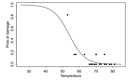
In January 1986, the space shuttle Challenger exploded shortly after launch. An investigation was launched into the cause of the crash and attention focused on the rubber O-ring seals in the rocket boosters. At lower temperatures, rubber becomes more brittle and is a less effective sealant. At the time of the launch, the temperature was $31^{\circ} \mathrm{F}$. Could the failure of the O-rings have been predicted? In the 23 previous shuttle missions for which data exists, some evidence of damage due to blow by and erosion was recorded on some O-rings. Each shuttle had two boosters, each with three O-rings. For each mission, we know the number of $\mathrm{O}$-rings out of six showing some damage and the launch temperature. This is a simplification of the problem see Dalal et al. (1989) for more details.
统计代写|广义线性模型代写generalized linear model代考|Inference
We use the same likelihood-based methods as in Section $2.3$ to derive the binomial deviance:
$$
D=2 \sum_{i=1}^{n}\left{y_{i} \log y_{i} / \hat{y}{i}+\left(m{i}-y_{i}\right) \log \left(m_{i}-y_{i}\right) /\left(m_{i}-\hat{y}{i}\right)\right} $$ where $\hat{y}{i}$ are the fitted values from the model.
Provided that $Y$ is truly binomial and that the $m_{i}$ are relatively large, the deviance is approximately $\chi^{2}$ distributed with $n-q-1$ degrees of freedom if the model is correct. Thus we can use the deviance to test whether the model is an adequate fit. For the logit model of the Challenger data, we may compute:
pchisq (deviance (1mod), df . residual (1mod), lower FALSE)
[1] $0.71641$
Since this $p$-value is well in excess of $0.05$, we conclude that this model fits sufficiently well. Of course, this does not mean that this model is correct or that a simpler model might not also fit adequately. Even so, for the null model:
pchisq $(38.9,22$, lower FALSE)
[1] $0.014489$
We see that the fit is inadequate, so we cannot ascribe the response to simple variation not dependent on any predictor. Note that a $\chi_{d}^{2}$ variable has mean $d$ and standard deviation $\sqrt{2 d}$ so that it is often possible to quickly judge whether a deviance is large or small without explicitly computing the $p$-value. If the deviance is far in excess of the degrees of freedom, the null hypothesis can be rejected.
The $\chi^{2}$ distribution is only an approximation that becomes more accurate as the $m_{i}$ increase. The approximation is very poor for small $m_{i}$ and fails entirely in binary cases where $m_{i}=1$. Although it is not possible to say exactly how large $m_{i}$ should be for an adequate approximation, $m_{i} \geq 5 \forall i$ has often been suggested. Permutation or bootstrap methods might be considered as an alternative.
We can also use the deviance to compare two models, with smaller model $S$ representing a subspace (usually a subset) of a larger model $L$. The likelihood ratio test statistic becomes $D_{S}-D_{L}$. This test statistic is asymptotically distributed $\chi_{l-s}^{2}$, assuming that the smaller model is correct and the distributional assumptions hold. We can use this to test the significance of temperature by computing the difference in the deviances between the model with and without temperature. The model without temperature is just the null model and the difference in degrees of freedom or parameters is one:
pchisq (38.9-16.9,1, lower=FALSE)
[1] $2.7265 \mathrm{e}-06$
广义线性模型代考
统计代写|广义线性模型代写generalized linear model代考|Estimation Problems
使用第 8.2 节中描述的 Fisher 评分算法估计逻辑回归模型通常很快。然而,有时也会出现困难。当收敛失败时,有时是由于以下数据集表现出的问题。我们采用著名的 Fisher Iris 数据的子集,仅考虑三种鸢尾花中的两种,并仅使用其中两种潜在的预测变量:
ibrary (dplyr)
irisr <- filter(iris, Species ! “virginica”) to ? 选择(萼片。宽度,
→萼片。长度,物种)
我们使用两个物种的不同形状的绘图符号绘制数据:
(p <- ggplot(irisr, aes (x=Sepa1. Width, y=Sepal.Length, shape=Species))
tgeom point ())
我们现在拟合一个逻辑回归模型,看看是否可以从两个萼片维度预测物种。
n−100p−3偏差−0.000零偏差−138.629(区别−138.629) 请注意,残差为零表示完美拟合,但由于高标准误差,所有预测变量均不显着。看一下数据就可以发现其中的原因。我们看到这两组是线性可分的,因此可以完美拟合。在这个例子中,我们遭受了财富的尴尬——我们可以完美地拟合数据。不幸的是,这会导致参数及其标准误差的估计不稳定,并且会(可能错误地)表明可以做出完美的预测。在这种情况下,可以考虑另一种拟合方法,称为精确逻辑回归。参见 Cox (1970) 或 Mehta 和 Patel (1995)。可以在 R 的 elrm 和 logistix 包中找到实现。
统计代写|广义线性模型代写generalized linear model代考|Binomial Regression Model
假设响应变量是一世为了一世=1,…,n是二项分布的乙(米一世,p一世)以便:
磷(是一世=是一世)=(米一世 是一世)p一世是一世(1−p一世)米一世−是一世
我们进一步假设是一世是独立的。构成响应的单个结果或试验是一世都受同样的约束q预测因子(X一世1,…,X一世q). 这组试验称为协变量类。例如,我们可能会记录特定类型的客户是否购买。按照惯例,一个结果被标记为成功(例如,在此示例中进行购买),而另一个结果被标记为失败。在这种情况下,不应该对成功和失败附加任何情感意义。例如,成功可能是患者死亡的标签,而生存则称为失败。因为我们需要对每个协变量类进行多次试验,所以二项式回归模型的数据更有可能来自设计的实验,其中一些预测变量处于选定的值,而不是可能更稀疏的观察数据。
与二进制情况一样,我们构造一个线性预测器:
这一世=b0+b1X一世1+⋯+bqX一世q
我们可以使用逻辑链接功能这一世=日志(p一世/(1−p一世)). 对数似然由下式给出:
l(b)=∑一世=1n[是一世这一世−米一世日志(1+和一世这)+日志(米一世 是一世)]
让我们通过一个示例来了解分析与二元响应案例的不同之处。
1986 年 1 月,挑战者号航天飞机在发射后不久爆炸。对坠机原因进行了调查,并将注意力集中在火箭助推器中的橡胶 O 形密封圈上。在较低温度下,橡胶变得更脆,并且是一种不太有效的密封剂。发射时气温为31∘F. O 形圈的故障是否可以预测?在有数据的之前的 23 次航天飞机任务中,一些 O 形环上记录了一些因吹漏和腐蚀而损坏的证据。每个航天飞机有两个助推器,每个助推器有三个 O 形环。对于每个任务,我们知道○- 六环显示一些损坏和发射温度。这是对问题的简化,请参见 Dalal 等人。(1989) 了解更多详情。
统计代写|广义线性模型代写generalized linear model代考|Inference
我们使用与第 1 节中相同的基于可能性的方法2.3导出二项式偏差:
D=2 \sum_{i=1}^{n}\left{y_{i} \log y_{i} / \hat{y}{i}+\left(m{i}-y_{i}\右) \log \left(m_{i}-y_{i}\right) /\left(m_{i}-\hat{y}{i}\right)\right}D=2 \sum_{i=1}^{n}\left{y_{i} \log y_{i} / \hat{y}{i}+\left(m{i}-y_{i}\右) \log \left(m_{i}-y_{i}\right) /\left(m_{i}-\hat{y}{i}\right)\right}在哪里是^一世是模型的拟合值。
前提是是是真正的二项式,并且米一世都比较大,偏差大约是χ2分布于n−q−1模型正确时的自由度。因此,我们可以使用偏差来测试模型是否合适。对于 Challenger 数据的 logit 模型,我们可以计算:
pchisq (deviance (1mod), df .residual (1mod), lower FALSE)
[1]0.71641
从此p-价值远远超过0.05,我们得出结论,该模型非常适合。当然,这并不意味着这个模型是正确的,或者更简单的模型也可能不适合。即便如此,对于空模型:
pchisq(38.9,22, 下 FALSE)
[1]0.014489
我们看到拟合不足,因此我们不能将响应归因于不依赖于任何预测变量的简单变化。请注意,一个χd2变量有均值d和标准差2d因此,通常可以快速判断偏差是大还是小,而无需明确计算p-价值。如果偏差远远超过自由度,则可以拒绝原假设。
这χ2分布只是一个近似值,随着米一世增加。对于小型的近似值很差米一世并且在二进制情况下完全失败米一世=1. 虽然无法确切地说出多大米一世应该是一个足够的近似值,米一世≥5∀一世经常被建议。置换或引导方法可能被视为一种替代方法。
我们也可以使用偏差来比较两个模型,较小的模型小号表示较大模型的子空间(通常是子集)大号. 似然比检验统计量变为D小号−D大号. 该检验统计量是渐近分布的χl−s2,假设较小的模型是正确的并且分布假设成立。我们可以通过计算有温度和没有温度的模型之间的偏差差异来使用它来测试温度的显着性。没有温度的模型只是空模型,自由度或参数的差异为一:
pchisq (38.9-16.9,1, lower=FALSE)
[1]2.7265和−06

统计代写请认准statistics-lab™. statistics-lab™为您的留学生涯保驾护航。
金融工程代写
金融工程是使用数学技术来解决金融问题。金融工程使用计算机科学、统计学、经济学和应用数学领域的工具和知识来解决当前的金融问题,以及设计新的和创新的金融产品。
非参数统计代写
非参数统计指的是一种统计方法,其中不假设数据来自于由少数参数决定的规定模型;这种模型的例子包括正态分布模型和线性回归模型。
广义线性模型代考
广义线性模型(GLM)归属统计学领域,是一种应用灵活的线性回归模型。该模型允许因变量的偏差分布有除了正态分布之外的其它分布。
术语 广义线性模型(GLM)通常是指给定连续和/或分类预测因素的连续响应变量的常规线性回归模型。它包括多元线性回归,以及方差分析和方差分析(仅含固定效应)。
有限元方法代写
有限元方法(FEM)是一种流行的方法,用于数值解决工程和数学建模中出现的微分方程。典型的问题领域包括结构分析、传热、流体流动、质量运输和电磁势等传统领域。
有限元是一种通用的数值方法,用于解决两个或三个空间变量的偏微分方程(即一些边界值问题)。为了解决一个问题,有限元将一个大系统细分为更小、更简单的部分,称为有限元。这是通过在空间维度上的特定空间离散化来实现的,它是通过构建对象的网格来实现的:用于求解的数值域,它有有限数量的点。边界值问题的有限元方法表述最终导致一个代数方程组。该方法在域上对未知函数进行逼近。[1] 然后将模拟这些有限元的简单方程组合成一个更大的方程系统,以模拟整个问题。然后,有限元通过变化微积分使相关的误差函数最小化来逼近一个解决方案。
tatistics-lab作为专业的留学生服务机构,多年来已为美国、英国、加拿大、澳洲等留学热门地的学生提供专业的学术服务,包括但不限于Essay代写,Assignment代写,Dissertation代写,Report代写,小组作业代写,Proposal代写,Paper代写,Presentation代写,计算机作业代写,论文修改和润色,网课代做,exam代考等等。写作范围涵盖高中,本科,研究生等海外留学全阶段,辐射金融,经济学,会计学,审计学,管理学等全球99%专业科目。写作团队既有专业英语母语作者,也有海外名校硕博留学生,每位写作老师都拥有过硬的语言能力,专业的学科背景和学术写作经验。我们承诺100%原创,100%专业,100%准时,100%满意。
随机分析代写
随机微积分是数学的一个分支,对随机过程进行操作。它允许为随机过程的积分定义一个关于随机过程的一致的积分理论。这个领域是由日本数学家伊藤清在第二次世界大战期间创建并开始的。
时间序列分析代写
随机过程,是依赖于参数的一组随机变量的全体,参数通常是时间。 随机变量是随机现象的数量表现,其时间序列是一组按照时间发生先后顺序进行排列的数据点序列。通常一组时间序列的时间间隔为一恒定值(如1秒,5分钟,12小时,7天,1年),因此时间序列可以作为离散时间数据进行分析处理。研究时间序列数据的意义在于现实中,往往需要研究某个事物其随时间发展变化的规律。这就需要通过研究该事物过去发展的历史记录,以得到其自身发展的规律。
回归分析代写
多元回归分析渐进(Multiple Regression Analysis Asymptotics)属于计量经济学领域,主要是一种数学上的统计分析方法,可以分析复杂情况下各影响因素的数学关系,在自然科学、社会和经济学等多个领域内应用广泛。
MATLAB代写
MATLAB 是一种用于技术计算的高性能语言。它将计算、可视化和编程集成在一个易于使用的环境中,其中问题和解决方案以熟悉的数学符号表示。典型用途包括:数学和计算算法开发建模、仿真和原型制作数据分析、探索和可视化科学和工程图形应用程序开发,包括图形用户界面构建MATLAB 是一个交互式系统,其基本数据元素是一个不需要维度的数组。这使您可以解决许多技术计算问题,尤其是那些具有矩阵和向量公式的问题,而只需用 C 或 Fortran 等标量非交互式语言编写程序所需的时间的一小部分。MATLAB 名称代表矩阵实验室。MATLAB 最初的编写目的是提供对由 LINPACK 和 EISPACK 项目开发的矩阵软件的轻松访问,这两个项目共同代表了矩阵计算软件的最新技术。MATLAB 经过多年的发展,得到了许多用户的投入。在大学环境中,它是数学、工程和科学入门和高级课程的标准教学工具。在工业领域,MATLAB 是高效研究、开发和分析的首选工具。MATLAB 具有一系列称为工具箱的特定于应用程序的解决方案。对于大多数 MATLAB 用户来说非常重要,工具箱允许您学习和应用专业技术。工具箱是 MATLAB 函数(M 文件)的综合集合,可扩展 MATLAB 环境以解决特定类别的问题。可用工具箱的领域包括信号处理、控制系统、神经网络、模糊逻辑、小波、仿真等。