如果你也在 怎样代写应用时间序列分析applied time series analysis这个学科遇到相关的难题,请随时右上角联系我们的24/7代写客服。
时间序列分析applied time series analysis是分析在一个时间间隔内收集的一系列数据点的具体方式。在时间序列分析applied time series analysis中,分析人员在设定的时间段内以一致的时间间隔记录数据点,而不仅仅是间歇性或随机地记录数据点。
statistics-lab™ 为您的留学生涯保驾护航 在代写应用时间序列分析applied time series analysis方面已经树立了自己的口碑, 保证靠谱, 高质且原创的统计Statistics代写服务。我们的专家在代写应用时间序列分析applied time series analysis方面经验极为丰富,各种代写应用时间序列分析applied time series analysis相关的作业也就用不着说。
我们提供的应用时间序列分析applied time series analysis及其相关学科的代写,服务范围广, 其中包括但不限于:
- Statistical Inference 统计推断
- Statistical Computing 统计计算
- Advanced Probability Theory 高等楖率论
- Advanced Mathematical Statistics 高等数理统计学
- (Generalized) Linear Models 广义线性模型
- Statistical Machine Learning 统计机器学习
- Longitudinal Data Analysis 纵向数据分析
- Foundations of Data Science 数据科学基础

统计代写|应用时间序列分析代写applied time series anakysis代考|STATIONARITY
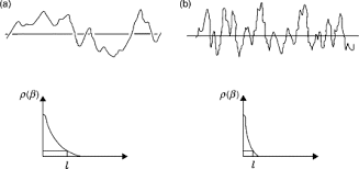
The foundation of time series analysis is stationarity. A time series $\left{r_{t}\right}$ is said to be strictly stationary if the joint distribution of $\left(r_{l_{1}}, \ldots, r_{t_{k}}\right)$ is identical to that of $\left(r_{t_{1}+1}, \ldots, r_{t_{k}+t}\right)$ for all $t$, where $k$ is an arbitrary positive integer and $\left(t_{1}, \ldots, t_{k}\right)$ is a collection of $k$ positive integers. In other words, strict stationarity requires that the joint distribution of $\left(r_{t_{1}}, \ldots, r_{t_{k}}\right)$ is invariant under time shift. This is a very strong condition that is hard to verify empirically. A weaker version of stationarity is often assumed. A time series $\left{r_{t}\right}$ is weakly stationary if both the mean of $r_{t}$ and the covariance between $r_{t}$ and $r_{t-\ell}$ are time-invariant, where $\ell$ is an arbitrary integer. More specifically, $\left{r_{t}\right}$ is weakly stationary if (a) $E\left(r_{l}\right)=\mu$, which is a constant, and (b) $\operatorname{Cov}\left(r_{t}, r_{t-\ell}\right)=\gamma_{\ell}$, which only depends on $\ell$. In practice, suppose that we have observed $T$ data points $\left{r_{t} \mid t=1, \ldots, T\right}$. The weak stationarity implies that the time plot of the data would show that the $T$ values fluctuate with constant variation around a constant level.
Implicitly in the condition of weak stationarity, we assume that the first two moments of $r_{t}$ are finite. From the definitions, if $r_{t}$ is strictly stationary and its first two moments are finite, then $r_{t}$ is also weakly stationary. The converse is not true in general. However, if the time series $r_{t}$ is normally distributed, then weak stationarity is equivalent to strict stationarity. In this book, we are mainly concerned with weakly stationary series.
The covariance $\gamma_{\ell}=\operatorname{Cov}\left(r_{t}, r_{t-\ell}\right)$ is called the lag- $\ell$ autocovariance of $r_{t}$. It has two important properties: (a) $\gamma_{0}=\operatorname{Var}\left(r_{t}\right)$ and (b) $\gamma_{-\ell}=\gamma_{\ell}$. The second property holds because $\operatorname{Cov}\left(r_{t}, r_{t-(-\ell)}\right)=\operatorname{Cov}\left(r_{t-(-\ell)}, r_{t}\right)=\operatorname{Cov}\left(r_{t+\ell}, r_{t}\right)=$ $\operatorname{Cov}\left(r_{t_{1}}, r_{l_{1}-\ell}\right)$, where $t_{1}=t+\ell$.
In the finance literature, it is common to assume that an asset return series is weakly stationary. This assumption can be checked empirically provided that a sufficient number of historical returns are available. For example, one can divide the data into subsamples and check the consistency of the results obtained.
统计代写|应用时间序列分析代写applied time series anakysis代考| CORRELATION AND AUTOCORRELATION FUNCTION
The correlation coefficient between two random variables $X$ and $Y$ is defined as
$$
\rho_{x, y}=\frac{\operatorname{Cov}(X, Y)}{\sqrt{\operatorname{Var}(X) \operatorname{Var}(Y)}}=\frac{E\left[\left(X-\mu_{x}\right)\left(Y-\mu_{y}\right)\right]}{\sqrt{E\left(X-\mu_{x}\right)^{2} E\left(Y-\mu_{y}\right)^{2}}},
$$
where $\mu_{x}$ and $\mu_{y}$ are the mean of $X$ and $Y$, respectively, and it is assumed that the variances exist. This coefficient measures the strength of linear dependence between $X$ and $Y$, and it can be shown that $-1 \leq \rho_{x, y} \leq 1$ and $\rho_{x, y}=\rho_{y, x}$. The two random variables are uncorrelated if $\rho_{x, y}=0$. In addition, if both $X$ and $Y$ are normal random variables, then $\rho_{x, y}=0$ if and only if $X$ and $Y$ are independent. When the sample $\left{\left(x_{l}, y_{t}\right)\right}_{t=1}^{T}$ is available, the correlation can be consistently estimated by its
sample counterpart
$$
\hat{\rho}{x, y}=\frac{\sum{t=1}^{T}\left(x_{t}-\bar{x}\right)\left(y_{t}-\bar{y}\right)}{\sqrt{\sum_{t=1}^{T}\left(x_{t}-\bar{x}\right)^{2} \sum_{t=1}^{T}\left(y_{t}-\bar{y}\right)^{2}}},
$$
where $\bar{x}=\sum_{t=1}^{T} x_{t} / T$ and $\bar{y}=\sum_{t=1}^{T} y_{t} / T$ are the sample mean of $X$ and $Y$, respectively.
统计代写|应用时间序列分析代写applied time series anakysis代考|Autocorrelation Function
Consider a weakly stationary return series $r_{t}$. When the linear dependence between $r_{t}$ and its past values $r_{t-i}$ is of interest, the concept of correlation is generalized to autocorrelation. The correlation coefficient between $r_{t}$ and $r_{t-\ell}$ is called the lag- $\ell$ autocorrelation of $r_{t}$ and is commonly denoted by $\rho_{\ell}$, which under the weak stationarity assumption is a function of $\ell$ only. Specifically, we define
$$
\rho_{\ell}=\frac{\operatorname{Cov}\left(r_{t}, r_{t-\ell}\right)}{\sqrt{\operatorname{Var}\left(r_{t}\right) \operatorname{Var}\left(r_{t-\ell}\right)}}=\frac{\operatorname{Cov}\left(r_{t}, r_{t-\ell}\right)}{\operatorname{Var}\left(r_{t}\right)}=\frac{\gamma_{\ell}}{\gamma_{0}},
$$
where the property $\operatorname{Var}\left(r_{t}\right)=\operatorname{Var}\left(r_{t-\ell}\right)$ for a weakly stationary series is used. From the definition, we have $\rho_{0}=1, \rho_{\ell}=\rho_{-\ell}$, and $-1 \leq \rho_{\ell} \leq 1$. In addition, a weakly stationary series $r_{t}$ is not serially correlated if and only if $\rho_{\ell}=0$ for all $\ell>0$.
For a given sample of returns $\left{r_{t}\right}_{t=1}^{T}$, let $\bar{r}$ be the sample mean (i.e., $\bar{r}=$ $\sum_{t=1}^{T} r_{t} / T$ ). Then the lag-1 sample autocorrelation of $r_{t}$ is
$$
\hat{\rho}{1}=\frac{\sum{t=2}^{T}\left(r_{t}-\bar{r}\right)\left(r_{t-1}-\bar{r}\right)}{\sum_{t=1}^{T}\left(r_{t}-\bar{r}\right)^{2}} .
$$
Under some general conditions, $\hat{\rho}{1}$ is a consistent estimate of $\rho{1}$. For example, if $\left{r_{t}\right}$ is an independent and identically distributed (iid) sequence and $E\left(r_{t}^{2}\right)<\infty$, then $\hat{\rho}{1}$ is asymptotically normal with mean zero and variance $1 / T$; see Brockwell and Davis (1991, Theorem 7.2.2). This result can be used in practice to test the null hypothesis $H{o}: \rho_{1}=0$ versus the alternative hypothesis $H_{a}: \rho_{1} \neq 0$. The test statistic is the usual $t$ ratio, which is $\sqrt{T} \hat{\rho}{1}$ and follows asymptotically the standard normal distribution. In general, the lag- $\ell$ sample autocorrelation of $r{t}$ is defined as $$ \hat{\rho}{\ell}=\frac{\sum{t=\ell+1}^{T}\left(r_{t}-\bar{r}\right)\left(r_{t-\ell}-\bar{r}\right)}{\sum_{t=1}^{T}\left(r_{t}-\bar{r}\right)^{2}}, \quad 0 \leq \ellq$. This is referred to as Bartlett’s formula in the time series literature; see Box, Jenkins, and Reinsel (1994). The previous
result can be used to perform the hypothesis testing of $H_{o}: \rho_{\ell}=0$ vs $H_{a}: \rho_{\ell} \neq 0$. For more information about the asymptotic distribution of sample autocorrelations, see Fuller (1976, Chapter 6) and Brockwell and Davis (1991, Chapter 7).
In finite samples, $\hat{\rho}{\ell}$ is a biased estimator of $\rho{\ell}$. The bias is in the order of $1 / T$, which can be substantial when the sample size $T$ is small. In most financial applications, $T$ is relatively large so that the bias is not serious.
时间序列分析代写
统计代写|应用时间序列分析代写applied time series anakysis代考|STATIONARITY
时间序列分析的基础是平稳性。一个时间序列\左{r_{t}\右}\左{r_{t}\右}如果联合分布是严格平稳的(rl1,…,r吨ķ)是相同的(r吨1+1,…,r吨ķ+吨)对全部吨, 在哪里ķ是任意正整数并且(吨1,…,吨ķ)是一个集合ķ正整数。换言之,严格平稳性要求(r吨1,…,r吨ķ)在时移下是不变的。这是一个非常强的条件,很难通过经验来验证。通常假设较弱的平稳性版本。一个时间序列\左{r_{t}\右}\左{r_{t}\右}如果两者的均值都是弱平稳的r吨和之间的协方差r吨和r吨−ℓ是时不变的,其中ℓ是任意整数。进一步来说,\左{r_{t}\右}\左{r_{t}\右}如果 (a) 是弱静止的和(rl)=μ,这是一个常数,并且 (b)这(r吨,r吨−ℓ)=Cℓ, 这仅取决于ℓ. 在实践中,假设我们已经观察到吨数据点\left{r_{t} \mid t=1, \ldots, T\right}\left{r_{t} \mid t=1, \ldots, T\right}. 弱平稳性意味着数据的时间图将表明吨值随着围绕恒定水平的恒定变化而波动。
在弱平稳性条件下,我们假设前两个矩r吨是有限的。根据定义,如果r吨是严格静止的并且它的前两个矩是有限的,那么r吨也是弱静止的。反之亦然。但是,如果时间序列r吨正态分布,则弱平稳性等价于严格平稳性。在本书中,我们主要关注弱平稳序列。
协方差Cℓ=这(r吨,r吨−ℓ)被称为滞后ℓ自协方差r吨. 它有两个重要的特性:(a)C0=曾是(r吨)(b)C−ℓ=Cℓ. 第二个属性成立,因为这(r吨,r吨−(−ℓ))=这(r吨−(−ℓ),r吨)=这(r吨+ℓ,r吨)= 这(r吨1,rl1−ℓ), 在哪里吨1=吨+ℓ.
在金融文献中,通常假设资产收益序列是弱平稳的。如果有足够数量的历史回报可用,则可以凭经验检验这一假设。例如,可以将数据分成子样本并检查所得结果的一致性。
统计代写|应用时间序列分析代写applied time series anakysis代考| CORRELATION AND AUTOCORRELATION FUNCTION
两个随机变量之间的相关系数X和是定义为
ρX,是=这(X,是)曾是(X)曾是(是)=和[(X−μX)(是−μ是)]和(X−μX)2和(是−μ是)2,
在哪里μX和μ是是平均值X和是, 并假设方差存在。该系数衡量之间线性相关的强度X和是, 并且可以证明−1≤ρX,是≤1和ρX,是=ρ是,X. 如果两个随机变量不相关ρX,是=0. 此外,如果两者X和是是正态随机变量,那么ρX,是=0当且仅当X和是是独立的。当样品\left{\left(x_{l}, y_{t}\right)\right}_{t=1}^{T}\left{\left(x_{l}, y_{t}\right)\right}_{t=1}^{T}是可用的,相关性可以通过其一致地估计
样品对应物
ρ^X,是=∑吨=1吨(X吨−X¯)(是吨−是¯)∑吨=1吨(X吨−X¯)2∑吨=1吨(是吨−是¯)2,
在哪里X¯=∑吨=1吨X吨/吨和是¯=∑吨=1吨是吨/吨是样本均值X和是, 分别。
统计代写|应用时间序列分析代写applied time series anakysis代考|Autocorrelation Function
考虑一个弱平稳的回报序列r吨. 当之间的线性依赖r吨及其过去的价值观r吨−一世有趣的是,相关的概念被推广到自相关。之间的相关系数r吨和r吨−ℓ被称为滞后ℓ的自相关r吨并且通常表示为ρℓ, 在弱平稳性假设下是ℓ只要。具体来说,我们定义
ρℓ=这(r吨,r吨−ℓ)曾是(r吨)曾是(r吨−ℓ)=这(r吨,r吨−ℓ)曾是(r吨)=CℓC0,
财产在哪里曾是(r吨)=曾是(r吨−ℓ)使用弱平稳序列。根据定义,我们有ρ0=1,ρℓ=ρ−ℓ, 和−1≤ρℓ≤1. 此外,弱平稳序列r吨当且仅当ρℓ=0对全部ℓ>0.
对于给定的回报样本\left{r_{t}\right}_{t=1}^{T}\left{r_{t}\right}_{t=1}^{T}, 让r¯是样本均值(即,r¯= ∑吨=1吨r吨/吨)。那么lag-1样本自相关r吨是
ρ^1=∑吨=2吨(r吨−r¯)(r吨−1−r¯)∑吨=1吨(r吨−r¯)2.
在一些一般情况下,ρ^1是一致的估计ρ1. 例如,如果\左{r_{t}\右}\左{r_{t}\右}是一个独立同分布 (iid) 序列,并且和(r吨2)<∞, 然后ρ^1是渐近正态的,均值为零和方差1/吨; 参见 Brockwell 和 Davis (1991, Theorem 7.2.2)。这个结果可以在实践中用来检验零假设H这:ρ1=0与备择假设H一种:ρ1≠0. 检验统计量是通常的吨比率,即吨ρ^1并且渐近地遵循标准正态分布。一般来说,滞后ℓ样本自相关r吨定义为 $$ \hat{\rho}{\ell}=\frac{\sum{t=\ell+1}^{T}\left(r_{t}-\bar{r}\right)\左(r_{t-\ell}-\bar{r}\right)}{\sum_{t=1}^{T}\left(r_{t}-\bar{r}\right)^{2 }}, \quad 0 \leq \ellq$。这在时间序列文献中被称为 Bartlett 公式;参见 Box、Jenkins 和 Reinsel (1994)。以前的
结果可用于执行假设检验H这:ρℓ=0对比H一种:ρℓ≠0. 有关样本自相关的渐近分布的更多信息,请参阅 Fuller(1976 年,第 6 章)和 Brockwell 和 Davis(1991 年,第 7 章)。
在有限样本中,ρ^ℓ是一个有偏估计量ρℓ. 偏差的顺序是1/吨,当样本量很大时,这可能很大吨是小。在大多数金融应用中,吨比较大,所以偏差不严重。

统计代写请认准statistics-lab™. statistics-lab™为您的留学生涯保驾护航。统计代写|python代写代考
随机过程代考
在概率论概念中,随机过程是随机变量的集合。 若一随机系统的样本点是随机函数,则称此函数为样本函数,这一随机系统全部样本函数的集合是一个随机过程。 实际应用中,样本函数的一般定义在时间域或者空间域。 随机过程的实例如股票和汇率的波动、语音信号、视频信号、体温的变化,随机运动如布朗运动、随机徘徊等等。
贝叶斯方法代考
贝叶斯统计概念及数据分析表示使用概率陈述回答有关未知参数的研究问题以及统计范式。后验分布包括关于参数的先验分布,和基于观测数据提供关于参数的信息似然模型。根据选择的先验分布和似然模型,后验分布可以解析或近似,例如,马尔科夫链蒙特卡罗 (MCMC) 方法之一。贝叶斯统计概念及数据分析使用后验分布来形成模型参数的各种摘要,包括点估计,如后验平均值、中位数、百分位数和称为可信区间的区间估计。此外,所有关于模型参数的统计检验都可以表示为基于估计后验分布的概率报表。
广义线性模型代考
广义线性模型(GLM)归属统计学领域,是一种应用灵活的线性回归模型。该模型允许因变量的偏差分布有除了正态分布之外的其它分布。
statistics-lab作为专业的留学生服务机构,多年来已为美国、英国、加拿大、澳洲等留学热门地的学生提供专业的学术服务,包括但不限于Essay代写,Assignment代写,Dissertation代写,Report代写,小组作业代写,Proposal代写,Paper代写,Presentation代写,计算机作业代写,论文修改和润色,网课代做,exam代考等等。写作范围涵盖高中,本科,研究生等海外留学全阶段,辐射金融,经济学,会计学,审计学,管理学等全球99%专业科目。写作团队既有专业英语母语作者,也有海外名校硕博留学生,每位写作老师都拥有过硬的语言能力,专业的学科背景和学术写作经验。我们承诺100%原创,100%专业,100%准时,100%满意。
机器学习代写
随着AI的大潮到来,Machine Learning逐渐成为一个新的学习热点。同时与传统CS相比,Machine Learning在其他领域也有着广泛的应用,因此这门学科成为不仅折磨CS专业同学的“小恶魔”,也是折磨生物、化学、统计等其他学科留学生的“大魔王”。学习Machine learning的一大绊脚石在于使用语言众多,跨学科范围广,所以学习起来尤其困难。但是不管你在学习Machine Learning时遇到任何难题,StudyGate专业导师团队都能为你轻松解决。
多元统计分析代考
基础数据: $N$ 个样本, $P$ 个变量数的单样本,组成的横列的数据表
变量定性: 分类和顺序;变量定量:数值
数学公式的角度分为: 因变量与自变量
时间序列分析代写
随机过程,是依赖于参数的一组随机变量的全体,参数通常是时间。 随机变量是随机现象的数量表现,其时间序列是一组按照时间发生先后顺序进行排列的数据点序列。通常一组时间序列的时间间隔为一恒定值(如1秒,5分钟,12小时,7天,1年),因此时间序列可以作为离散时间数据进行分析处理。研究时间序列数据的意义在于现实中,往往需要研究某个事物其随时间发展变化的规律。这就需要通过研究该事物过去发展的历史记录,以得到其自身发展的规律。
回归分析代写
多元回归分析渐进(Multiple Regression Analysis Asymptotics)属于计量经济学领域,主要是一种数学上的统计分析方法,可以分析复杂情况下各影响因素的数学关系,在自然科学、社会和经济学等多个领域内应用广泛。
MATLAB代写
MATLAB 是一种用于技术计算的高性能语言。它将计算、可视化和编程集成在一个易于使用的环境中,其中问题和解决方案以熟悉的数学符号表示。典型用途包括:数学和计算算法开发建模、仿真和原型制作数据分析、探索和可视化科学和工程图形应用程序开发,包括图形用户界面构建MATLAB 是一个交互式系统,其基本数据元素是一个不需要维度的数组。这使您可以解决许多技术计算问题,尤其是那些具有矩阵和向量公式的问题,而只需用 C 或 Fortran 等标量非交互式语言编写程序所需的时间的一小部分。MATLAB 名称代表矩阵实验室。MATLAB 最初的编写目的是提供对由 LINPACK 和 EISPACK 项目开发的矩阵软件的轻松访问,这两个项目共同代表了矩阵计算软件的最新技术。MATLAB 经过多年的发展,得到了许多用户的投入。在大学环境中,它是数学、工程和科学入门和高级课程的标准教学工具。在工业领域,MATLAB 是高效研究、开发和分析的首选工具。MATLAB 具有一系列称为工具箱的特定于应用程序的解决方案。对于大多数 MATLAB 用户来说非常重要,工具箱允许您学习和应用专业技术。工具箱是 MATLAB 函数(M 文件)的综合集合,可扩展 MATLAB 环境以解决特定类别的问题。可用工具箱的领域包括信号处理、控制系统、神经网络、模糊逻辑、小波、仿真等。