如果你也在 怎样代写应用统计applied statistics这个学科遇到相关的难题,请随时右上角联系我们的24/7代写客服。
应用统计学包括计划收集数据,管理数据,分析、解释和从数据中得出结论,以及利用分析结果确定问题、解决方案和机会。本专业培养学生在数据分析和实证研究方面的批判性思维和解决问题的能力。
statistics-lab™ 为您的留学生涯保驾护航 在代写应用统计applied statistics方面已经树立了自己的口碑, 保证靠谱, 高质且原创的统计Statistics代写服务。我们的专家在代写应用统计applied statistics代写方面经验极为丰富,各种代写应用统计applied statistics相关的作业也就用不着说。
我们提供的应用统计applied statistics及其相关学科的代写,服务范围广, 其中包括但不限于:
- Statistical Inference 统计推断
- Statistical Computing 统计计算
- Advanced Probability Theory 高等概率论
- Advanced Mathematical Statistics 高等数理统计学
- (Generalized) Linear Models 广义线性模型
- Statistical Machine Learning 统计机器学习
- Longitudinal Data Analysis 纵向数据分析
- Foundations of Data Science 数据科学基础
统计代写|应用统计代写applied statistics代考|Histograms and density plots
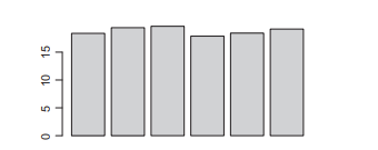
By default, if you plot just a single continuous variable using $q$ plot( $), R$ will plot a histogram (Figure 4.5, left). Histograms are extremely useful for seeing the distribution of your data. Do they look normally distributed? Are they skewed to one side or the other? There is technically no need to specify a “geom” here, but I think it is a good idea to be clear in your code, so I would recommend it.
Make a basic histogram
ac-qplot (data=Rxp. clean
$\mathrm{x}=$ Mass . final,
geom $=$ “histogram”)
The same principle of using the color or fill arguments as a way to view your data apply to histograms, but with one caveat. If you add a fill or color argument to a histogram in qplot ()$, \mathrm{R}$ will make a stacked histogram (Figure 4.5, middle). It can be more useful to see the data distributions overlayed on one another. This is best achieved with a density plot, which is similar to a histogram but instead plots a smoothed line that shows the shape of the data (Figure 4.5, right). Note that you should use the “col” argument in the density plot instead of the “fill” argument. What happens if you do not?
Hake a stacked histogram
be-qplot (data=RxP. clean,
$x=$ Mass.final,
geom=”histogram”,
Make a stacked histogram,
be-qplot (data=RxP.clean,
x=Mass. final,
geom= “histogram”,
fill=Pred)
Make overlayed density plots
ce-qplot (data=RxP. clean,
x=Mass.final,
geom=”density”,
fill=Pred)
#Make overlayed density plots
ce-qplot (data=RxP. clean,
$x=$ Mass. final,
geoms “density”,
统计代写|应用统计代写applied statistics代考|Scatterplots
The same principle works for continuous response variables. Previously, we defined our $\mathrm{x}$-axis as a categorical variable, but if we instead use a continuous variable $\mathrm{R}$ will plot a scatterplot. We can still use facets or colors to visualize the variation in our data, which is extremely useful. For example, in the following code I’ve filled the points based on the resource treatment, and faceted the data based on the predator treatment. Imagine the possibilities (Figure 4.6)!
Hake a serles of scatter plots
qplot (data=RxP. clean,
$x=\log$ (SVL. final),
Make a series of scatter
qplot (data=RxP. clean,
$\mathrm{x}=\log ($ SvL. final),
$\mathrm{y}=\log$ (Mass. final),
col=Res,
facets=. – Pred)
$y=\log ($ Mass. final),
col=Res,
facets=.-Pred)
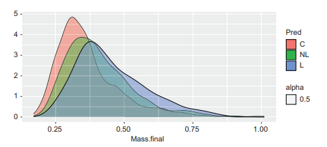
Note that when we make a plot like this, many of the points end up on top of one another, making it difficult to see all the data. We can add an argument to set the alpha level, or the degree of translucency of the points to alleviate this issue. This is also particularly useful with density plots. For example, we can remake the density plots from above, but this time we will fill them instead of color them and set the alpha to be $0.5$ (Figure $4.7$ ).
qplot (data=RxP. clean,
$x=$ Mass . final,
geom=” density”,
fill=pred,
alpha $=0.5$ )
Note that setting the alpha level in qplot() makes the alpha level $50 \%$ transparent, no matter what value you enter. I will show you how to set it to whatever you want later.
In addition to visualizing our data by setting the fill or color to one of our variables, we can also change the shape of the points based on a variable in our data frame with the “shape $=$ ” argument (Figure 4.8).
Hake a series of scatter plots
qplot (data =kxp. clean,
Mke a series of scatter plots
qplot (data=RxP. clean,
x=log(SVL. final).
$x=\log$ (SVL. final),
统计代写|应用统计代写applied statistics代考|PLOTTING YOUR DATA
In Chapter 3, we saw how to use functions from the dplyr package to summarize our data and we produced a tibble called RP.means that contained the means and standard errors for SVL.initial for each combination of resource and predator treatments. Now, we will see how to take those summarized data and turn them into a nice looking figure. In particular, we are going to make a bar graph. Why a bar graph you ask? There are several reasons really. First, despite their ubiquity in publications, the R gurus do not like bar graphs (or barplots, as we will call them) and making one is kind of a pain in $\mathrm{R}$. This is because bar graphs have an ability to hide a lot about your data (they just show the mean and whatever your error bar of choice is). But the fact that they are difficult to create makes them an excellent tool for teaching many of the ways you can, and probably should, customize your figures. That said, box plots are much more informative and are finally becoming increasingly used in published science. The second reason is that despite their downsides many people still like bar graphs and want to make them, so it is useful to know how to make one.
The most basic function to make a bar graph is barplot(). There are many, many arguments that can be passed to barplot(), which can be viewed in the help file (remember how to get to the help: ?barplot). A slightly improved version is the function barplot2(), which makes plotting error bars much simpler. barplot2() is found in the gplots package. You can also make a barplot in ggplot2. We will go through both examples. I find it useful and instructive to demonstrate the older technique using base graphics first, as it demonstrates how you can modify every little thing in a figure in R. Much of the coding techniques are also useful in ggplot2, and we will use ggplot2 for most everything in this book. If you feel confident
you will never, ever, ever use base graphics, feel free to skip ahead a few pages to the section on ggplot2. However, if you want to learn a little more about $\mathrm{R}$ and customizing figures, I encourage you to follow along with the next few pages of commands.
4.3.1 Making a barplot in base graphics
Let’s start by simply plotting the bars in their most basic form. Note that I am assuming you still have the RPmeans object we created in Chapter $3 .$
应用统计代写
统计代写|应用统计代写applied statistics代考|Histograms and density plots
默认情况下,如果您只绘制一个连续变量,使用q阴谋(),R将绘制一个直方图(图 4.5,左)。直方图对于查看数据的分布非常有用。它们看起来是正态分布的吗?他们偏向一侧还是另一侧?从技术上讲,这里不需要指定“geom”,但我认为在你的代码中清晰是个好主意,所以我会推荐它。
制作基本直方图
ac-qplot (data=Rxp.clean
X=大量的 。最后,
几何=“直方图”)
使用颜色或填充参数作为查看数据的方式的相同原则适用于直方图,但有一个警告。如果在 qplot() 中为直方图添加填充或颜色参数,R将制作一个堆叠直方图(图 4.5,中间)。查看相互叠加的数据分布可能更有用。最好使用密度图来实现这一点,它类似于直方图,而是绘制一条显示数据形状的平滑线(图 4.5,右)。请注意,您应该在密度图中使用“col”参数而不是“fill”参数。如果不这样做会怎样?
绘制堆叠直方图
be-qplot (data=RxP.clean,
X=Mass.final,
geom=”histogram”,
制作堆叠直方图,
be-qplot(数据=RxP.clean,
x=Mass.final,
geom=“直方图”,
填充=Pred)
制作叠加密度图
ce-qplot (data=RxP. clean,
x=Mass.final,
geom=”density”,
fill=Pred) #制作
叠加密度图
ce-qplot (data=RxP. clean,
X=质量最终,
几何“密度”,
统计代写|应用统计代写applied statistics代考|Scatterplots
同样的原理也适用于连续响应变量。之前,我们定义了我们的X-axis 作为分类变量,但如果我们改为使用连续变量R将绘制散点图。我们仍然可以使用构面或颜色来可视化数据的变化,这非常有用。例如,在下面的代码中,我根据资源处理填充了点,并根据捕食者处理对数据进行了分面。想象一下可能性(图 4.6)!
获得一系列散点图
qplot (data=RxP.clean,
X=日志(SVL。最终),
制作一系列散点图
qplot(数据=RxP。干净,
X=日志(SVL。最终的),
是=日志(质量。最终),
col=Res,
facets=。– 预测)
是=日志(Mass.final),
col=Res,
facets=.-Pred)
请注意,当我们制作这样的图时,许多点最终会相互重叠,因此很难查看所有数据。我们可以添加一个参数来设置 alpha 级别,或者点的半透明程度来缓解这个问题。这对于密度图也特别有用。例如,我们可以从上面重新制作密度图,但这次我们将填充它们而不是着色它们并将 alpha 设置为0.5(数字4.7)。
qplot(数据=RxP。干净,
X=大量的 。最终,
geom=“密度”,
填充=pred,
alpha=0.5)
请注意,在 qplot() 中设置 alpha 级别会使 alpha 级别50%透明,无论您输入什么值。稍后我将向您展示如何将其设置为您想要的任何内容。
除了通过将填充或颜色设置为我们的变量之一来可视化我们的数据之外,我们还可以根据数据框中的变量来更改点的形状,其中“形状=” 论点(图 4.8)。
Hake 一系列散点图
qplot (data =kxp.clean,
制作一系列散点图
qplot(数据=RxP.clean,
x=log(SVL.final)。
X=日志(SVL。最终),
统计代写|应用统计代写applied statistics代考|PLOTTING YOUR DATA
在第 3 章中,我们看到了如何使用 dplyr 包中的函数来总结我们的数据,我们生成了一个名为 RP.means 的 tibble,其中包含 SVL.initial 对于每种资源和捕食者处理组合的均值和标准误差。现在,我们将了解如何获取这些汇总数据并将它们变成一个漂亮的图形。特别是,我们将制作一个条形图。你问为什么是条形图?确实有几个原因。首先,尽管它们在出版物中无处不在,但 R 大师们不喜欢条形图(或我们称之为条形图),制作一个是一种痛苦R. 这是因为条形图能够隐藏很多关于您的数据的能力(它们只显示平均值以及您选择的误差条)。但它们难以创建的事实使它们成为教授许多您可以并且可能应该自定义图形的方法的绝佳工具。也就是说,箱形图的信息量要大得多,并且最终在已发表的科学中越来越多地使用。第二个原因是尽管有缺点,但许多人仍然喜欢条形图并想要制作它们,因此知道如何制作它很有用。
制作条形图最基本的函数是 barplot()。有很多很多参数可以传递给 barplot(),可以在帮助文件中查看(记住如何获得帮助:?barplot)。稍微改进的版本是函数 barplot2(),它使绘制误差线更加简单。barplot2() 位于 gplots 包中。您还可以在 ggplot2 中制作条形图。我们将通过这两个例子。我发现首先使用基础图形演示旧技术很有用且具有启发性,因为它演示了如何修改 R 中图形中的每一个小东西。许多编码技术在 ggplot2 中也很有用,我们将在大多数情况下使用 ggplot2本书中的一切。如果你感到自信
你永远永远不会使用基本图形,请随意跳过几页到 ggplot2 部分。但是,如果您想了解更多关于R和自定义图形,我鼓励您按照接下来的几页命令进行操作。
4.3.1 在基本图形中制作条形图
让我们从简单地以最基本的形式绘制条形图开始。请注意,我假设您仍然拥有我们在第 1 章中创建的 RPmeans 对象3.

统计代写请认准statistics-lab™. statistics-lab™为您的留学生涯保驾护航。
金融工程代写
金融工程是使用数学技术来解决金融问题。金融工程使用计算机科学、统计学、经济学和应用数学领域的工具和知识来解决当前的金融问题,以及设计新的和创新的金融产品。
非参数统计代写
非参数统计指的是一种统计方法,其中不假设数据来自于由少数参数决定的规定模型;这种模型的例子包括正态分布模型和线性回归模型。
广义线性模型代考
广义线性模型(GLM)归属统计学领域,是一种应用灵活的线性回归模型。该模型允许因变量的偏差分布有除了正态分布之外的其它分布。
术语 广义线性模型(GLM)通常是指给定连续和/或分类预测因素的连续响应变量的常规线性回归模型。它包括多元线性回归,以及方差分析和方差分析(仅含固定效应)。
有限元方法代写
有限元方法(FEM)是一种流行的方法,用于数值解决工程和数学建模中出现的微分方程。典型的问题领域包括结构分析、传热、流体流动、质量运输和电磁势等传统领域。
有限元是一种通用的数值方法,用于解决两个或三个空间变量的偏微分方程(即一些边界值问题)。为了解决一个问题,有限元将一个大系统细分为更小、更简单的部分,称为有限元。这是通过在空间维度上的特定空间离散化来实现的,它是通过构建对象的网格来实现的:用于求解的数值域,它有有限数量的点。边界值问题的有限元方法表述最终导致一个代数方程组。该方法在域上对未知函数进行逼近。[1] 然后将模拟这些有限元的简单方程组合成一个更大的方程系统,以模拟整个问题。然后,有限元通过变化微积分使相关的误差函数最小化来逼近一个解决方案。
tatistics-lab作为专业的留学生服务机构,多年来已为美国、英国、加拿大、澳洲等留学热门地的学生提供专业的学术服务,包括但不限于Essay代写,Assignment代写,Dissertation代写,Report代写,小组作业代写,Proposal代写,Paper代写,Presentation代写,计算机作业代写,论文修改和润色,网课代做,exam代考等等。写作范围涵盖高中,本科,研究生等海外留学全阶段,辐射金融,经济学,会计学,审计学,管理学等全球99%专业科目。写作团队既有专业英语母语作者,也有海外名校硕博留学生,每位写作老师都拥有过硬的语言能力,专业的学科背景和学术写作经验。我们承诺100%原创,100%专业,100%准时,100%满意。
随机分析代写
随机微积分是数学的一个分支,对随机过程进行操作。它允许为随机过程的积分定义一个关于随机过程的一致的积分理论。这个领域是由日本数学家伊藤清在第二次世界大战期间创建并开始的。
时间序列分析代写
随机过程,是依赖于参数的一组随机变量的全体,参数通常是时间。 随机变量是随机现象的数量表现,其时间序列是一组按照时间发生先后顺序进行排列的数据点序列。通常一组时间序列的时间间隔为一恒定值(如1秒,5分钟,12小时,7天,1年),因此时间序列可以作为离散时间数据进行分析处理。研究时间序列数据的意义在于现实中,往往需要研究某个事物其随时间发展变化的规律。这就需要通过研究该事物过去发展的历史记录,以得到其自身发展的规律。
回归分析代写
多元回归分析渐进(Multiple Regression Analysis Asymptotics)属于计量经济学领域,主要是一种数学上的统计分析方法,可以分析复杂情况下各影响因素的数学关系,在自然科学、社会和经济学等多个领域内应用广泛。
MATLAB代写
MATLAB 是一种用于技术计算的高性能语言。它将计算、可视化和编程集成在一个易于使用的环境中,其中问题和解决方案以熟悉的数学符号表示。典型用途包括:数学和计算算法开发建模、仿真和原型制作数据分析、探索和可视化科学和工程图形应用程序开发,包括图形用户界面构建MATLAB 是一个交互式系统,其基本数据元素是一个不需要维度的数组。这使您可以解决许多技术计算问题,尤其是那些具有矩阵和向量公式的问题,而只需用 C 或 Fortran 等标量非交互式语言编写程序所需的时间的一小部分。MATLAB 名称代表矩阵实验室。MATLAB 最初的编写目的是提供对由 LINPACK 和 EISPACK 项目开发的矩阵软件的轻松访问,这两个项目共同代表了矩阵计算软件的最新技术。MATLAB 经过多年的发展,得到了许多用户的投入。在大学环境中,它是数学、工程和科学入门和高级课程的标准教学工具。在工业领域,MATLAB 是高效研究、开发和分析的首选工具。MATLAB 具有一系列称为工具箱的特定于应用程序的解决方案。对于大多数 MATLAB 用户来说非常重要,工具箱允许您学习和应用专业技术。工具箱是 MATLAB 函数(M 文件)的综合集合,可扩展 MATLAB 环境以解决特定类别的问题。可用工具箱的领域包括信号处理、控制系统、神经网络、模糊逻辑、小波、仿真等。