如果你也在 怎样代写强化学习Reinforcement Learning这个学科遇到相关的难题,请随时右上角联系我们的24/7代写客服。
强化学习是一种基于奖励期望行为和/或惩罚不期望行为的机器学习训练方法。一般来说,强化学习代理能够感知和解释其环境,采取行动并通过试验和错误学习。
statistics-lab™ 为您的留学生涯保驾护航 在代写强化学习Reinforcement Learning方面已经树立了自己的口碑, 保证靠谱, 高质且原创的统计Statistics代写服务。我们的专家在代写强化学习Reinforcement Learning代写方面经验极为丰富,各种代写强化学习Reinforcement Learning相关的作业也就用不着说。
我们提供的强化学习Reinforcement Learning及其相关学科的代写,服务范围广, 其中包括但不限于:
- Statistical Inference 统计推断
- Statistical Computing 统计计算
- Advanced Probability Theory 高等楖率论
- Advanced Mathematical Statistics 高等数理统计学
- (Generalized) Linear Models 广义线性模型
- Statistical Machine Learning 统计机器学习
- Longitudinal Data Analysis 纵向数据分析
- Foundations of Data Science 数据科学基础
统计代写|强化学习作业代写Reinforcement Learning代考|Prediction with Monte Carlo
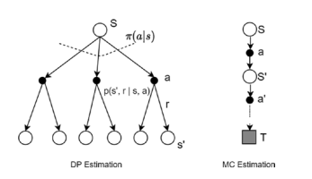
When we do not know the model dynamics, what do we do? Think back to a situation when you did not know something about a problem. What did you do in that situation? You experiment, take some steps, and find out how the situation responds. For example, say you want to find out if a die or a coin is biased or not. You toss the coin or throw the die multiple times, observe the outcome, and use that to form your opinion. In other words, you sample. The law of large numbers from statistics tell us that the average of samples is a good substitute for the averages. Further, these averages become better as the number of samples increase. If you look back at the Bellman equations in the previous chapter, you will notice that we had expectation operator $\mathrm{E}[\cdot]$ in those equations; e.g., the value of a state being $v(s)=E\left[G_{t} \mid S_{t}=s\right]$. Further, to calculate $v(s)$, we used dynamic programming requiring the transition dynamics $p(s, r \mid s, a)$. In the absence of the model dynamics knowledge, what do we do? We just sample from the model, observing returns starting from state $S=s$ and until the end of the episode. We then average the returns from all episode runs and use that average as an estimate of $v_{\pi}(s)$ for the policy $\pi$ that the agent is following. This in a nutshell is the approach of Monte Carlo methods: replace expected returns with the average of sample returns.
There are a few points to note. MC methods do not require knowledge of the model. The only thing required is that we should be able to sample from it. We need to know the return of starting from a state until termination, and hence we can use MC methods only on episodic MDPs in which every run finally terminates. It will not work on nonterminating environments. The second point is that for a large MDP we can keep the focus on sampling only that part of the MDP that is relevant and avoid exploring irrelevant parts of the MDP. Such an approach makes MC methods highly scalable for very large problems. A variant of the MC method called Monte Carlo tree search (MCTS) was used by OpenAI in training a Go game-playing agent.
统计代写|强化学习作业代写Reinforcement Learning代考|Bias and Variance of MC Predication Methods
Let’s now look at the pros and cons of “first visit” versus “every visit.” Do both of them converge to the true underlying $V(s)$ ? Do they fluctuate a lot while converging? Does one converge faster to true value? Before we answer this question, let’s first review the basic concept of bias-variance trade-off that we see in all statistical model estimations, e.g., in supervised learning.
Bias refers to the property of the model to converge to the true underlying value that we are trying to estimate, in our case $v_{\pi}(s)$. Some estimators are biased, meaning they are not able to converge to the true value due to their inherent lack of flexibility, i.e., being too simple or restricted for a given true model. At the same time, in some other cases, models have bias that goes down to zero as the number of samples grows.
Variance refers to the model estimate being sensitive to the specific sample data being used. This means the estimate value may fluctuate a lot and hence may require a large data set or trials for the estimate average to converge to a stable value.
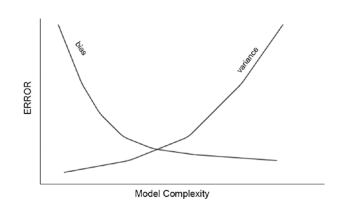
The models, which are very flexible, have low bias as they are able to fit the model to any configuration of a data set. At the same time, due to flexibility, they can overfit to the data, making the estimates vary a lot as the training data changes. On the other hand, models that are simpler have high bias. Such models, due to the inherent simplicity and restrictions, may not be able to represent the true underlying model. But they will also have low variance as they do not overfit. This is known as bias-variance trade-off and can be presented in a graph as shown in Figure 4-3.
统计代写|强化学习作业代写Reinforcement Learning代考|Control with Monte Carlo
Let’s now talk about control in a model-free setup. We need to find the optimal policy in this setup without knowing the model dynamics. As a refresher, let’s look at the generalized policy iteration (GPI) that was introduced in Chapter 3. In GPI, we iterate between two steps. The first step is to find the state values for a given policy, and the second step is to improve the policy using greedy optimization. We will follow the same GPI approach for control under MC. We will have some tweaks, though, to account for the fact that we are in model-free world with no access/knowledge of transition dynamics.
In Chapter 3 , we looked at state values, $v(s)$. However, in the absence of transition dynamics, state values alone will not be sufficient. For the greedy improvement step, we need access to the action values, $q(s, a)$. We need to know the q-values for all possible actions, i.e., all $q(S=s, a)$ for all possible actions $a$ in state $S=s$. Only with that information will we be able to apply a greedy maximization to pick the best action, i.e., $\operatorname{argmax}_{\mathrm{a}} q(\mathrm{~s}, a)$. $^{2}$
We have another complication when compared to DP. The agent follows a policy at the time of generating the samples. However, such a policy may result in many stateaction pairs never being visited, and even more so if the policy is a deterministic one. If the agent does not visit a state-action pair, it does not know all $q(s, a)$ for a given state, and hence it cannot find the maximum q-value yielding an action. One way to solve the issue is to ensure enough exploration by exploring starts, i.e., ensuring that the agent starts an episode from a random state-action pair and over the course of many episodes covers each state-action pair enough times, in fact, infinite in limit.
Figure 4-4 shows the GPI diagram with the change of $v$-values to $q$-values. The evaluation step now is the MC prediction step that was introduced in the previous section. Once the q-values stabilize, greedy maximization can be applied to obtain a new policy. The policy improvement theorem ensures that the new policy will be better or at least as good as the old policy. The previous approach of GPI will be a recurring theme. Based on the setup, the evaluation steps will change, and the improvement step invariably will continue to be greedy maximization.
强化学习代写
统计代写|强化学习作业代写Reinforcement Learning代考|Prediction with Monte Carlo
当我们不知道模型动力学时,我们该怎么办?回想一下您对某个问题一无所知的情况。在那种情况下你做了什么?您进行实验,采取一些步骤,并找出情况如何反应。例如,假设您想知道骰子或硬币是否有偏差。您多次掷硬币或掷骰子,观察结果,并以此形成您的意见。换句话说,你采样。统计中的大数定律告诉我们,样本的平均值可以很好地替代平均值。此外,随着样本数量的增加,这些平均值会变得更好。如果你回顾上一章的贝尔曼方程,你会注意到我们有期望算子和[⋅]在那些方程中;例如,一个状态的值是在(s)=和[G吨∣小号吨=s]. 此外,要计算在(s),我们使用需要过渡动态的动态规划p(s,r∣s,一种). 在没有模型动力学知识的情况下,我们该怎么办?我们只是从模型中采样,观察从状态开始的回报小号=s直到这一集结束。然后,我们平均所有剧集运行的回报,并使用该平均值作为在圆周率(s)为政策圆周率代理正在跟踪。简而言之,这就是蒙特卡洛方法的方法:用样本收益的平均值代替预期收益。
有几点需要注意。MC 方法不需要模型知识。唯一需要的是我们应该能够从中取样。我们需要知道从一个状态开始到终止的返回,因此我们只能在每次运行最终终止的情节 MDP 上使用 MC 方法。它不适用于非终止环境。第二点是,对于大型 MDP,我们可以将重点放在仅对 MDP 中相关的部分进行采样,而避免探索 MDP 中不相关的部分。这种方法使得 MC 方法对于非常大的问题具有高度可扩展性。OpenAI 使用称为蒙特卡洛树搜索 (MCTS) 的 MC 方法的一种变体来训练围棋游戏代理。
统计代写|强化学习作业代写Reinforcement Learning代考|Bias and Variance of MC Predication Methods
现在让我们看看“首次访问”与“每次访问”的优缺点。它们都收敛到真正的底层吗在(s)? 它们在收敛时波动很大吗?一个人会更快地收敛到真实值吗?在我们回答这个问题之前,让我们首先回顾一下我们在所有统计模型估计中看到的偏差-方差权衡的基本概念,例如在监督学习中。
在我们的例子中,偏差是指模型收敛到我们试图估计的真实基础价值的属性在圆周率(s). 一些估计器是有偏差的,这意味着由于它们固有的缺乏灵活性,即对于给定的真实模型过于简单或受限,它们无法收敛到真实值。同时,在其他一些情况下,随着样本数量的增加,模型的偏差会下降到零。
方差是指模型估计对所使用的特定样本数据敏感。这意味着估计值可能会波动很大,因此可能需要大量数据集或试验才能使估计平均值收敛到稳定值。
这些模型非常灵活,具有低偏差,因为它们能够使模型适应数据集的任何配置。同时,由于灵活性,它们可以对数据进行过拟合,使得估计值随着训练数据的变化而变化很大。另一方面,更简单的模型具有高偏差。由于固有的简单性和限制,此类模型可能无法代表真正的基础模型。但它们也将具有低方差,因为它们不会过度拟合。这被称为偏差-方差权衡,可以在图 4-3 中显示。
统计代写|强化学习作业代写Reinforcement Learning代考|Control with Monte Carlo
现在让我们谈谈无模型设置中的控制。我们需要在不知道模型动态的情况下找到此设置中的最优策略。作为复习,让我们看一下第 3 章中介绍的广义策略迭代(GPI)。在 GPI 中,我们在两个步骤之间进行迭代。第一步是找到给定策略的状态值,第二步是使用贪心优化改进策略。在 MC 下,我们将遵循相同的 GPI 方法进行控制。不过,我们将进行一些调整,以说明我们处于无模型世界,无法访问/了解过渡动态这一事实。
在第 3 章中,我们研究了状态值,在(s). 然而,在没有过渡动态的情况下,仅靠状态值是不够的。对于贪心改进步骤,我们需要访问动作值,q(s,一种). 我们需要知道所有可能动作的 q 值,即所有q(小号=s,一种)对于所有可能的动作一种处于状态小号=s. 只有有了这些信息,我们才能应用贪心最大化来选择最佳行动,即最大参数一种q( s,一种). 2
与 DP 相比,我们还有另一个问题。代理在生成样本时遵循策略。但是,这样的策略可能会导致许多状态动作对永远不会被访问,如果策略是确定性的,则更是如此。如果代理不访问状态-动作对,它不知道所有q(s,一种)对于给定的状态,因此它无法找到产生动作的最大 q 值。解决这个问题的一种方法是通过探索开始来确保足够的探索,即确保代理从随机状态-动作对开始一个情节,并且在许多情节的过程中足够多次地覆盖每个状态-动作对,事实上,无限的极限。
图 4-4 显示了 GPI 图随着在-值到q-价值观。现在的评估步骤是上一节中介绍的 MC 预测步骤。一旦 q 值稳定,就可以应用贪心最大化来获得新策略。策略改进定理确保新策略将更好或至少与旧策略一样好。GPI 以前的方法将是一个反复出现的主题。根据设置,评估步骤会发生变化,而改进步骤总是会继续贪婪最大化。

统计代写请认准statistics-lab™. statistics-lab™为您的留学生涯保驾护航。
金融工程代写
金融工程是使用数学技术来解决金融问题。金融工程使用计算机科学、统计学、经济学和应用数学领域的工具和知识来解决当前的金融问题,以及设计新的和创新的金融产品。
非参数统计代写
非参数统计指的是一种统计方法,其中不假设数据来自于由少数参数决定的规定模型;这种模型的例子包括正态分布模型和线性回归模型。
广义线性模型代考
广义线性模型(GLM)归属统计学领域,是一种应用灵活的线性回归模型。该模型允许因变量的偏差分布有除了正态分布之外的其它分布。
术语 广义线性模型(GLM)通常是指给定连续和/或分类预测因素的连续响应变量的常规线性回归模型。它包括多元线性回归,以及方差分析和方差分析(仅含固定效应)。
有限元方法代写
有限元方法(FEM)是一种流行的方法,用于数值解决工程和数学建模中出现的微分方程。典型的问题领域包括结构分析、传热、流体流动、质量运输和电磁势等传统领域。
有限元是一种通用的数值方法,用于解决两个或三个空间变量的偏微分方程(即一些边界值问题)。为了解决一个问题,有限元将一个大系统细分为更小、更简单的部分,称为有限元。这是通过在空间维度上的特定空间离散化来实现的,它是通过构建对象的网格来实现的:用于求解的数值域,它有有限数量的点。边界值问题的有限元方法表述最终导致一个代数方程组。该方法在域上对未知函数进行逼近。[1] 然后将模拟这些有限元的简单方程组合成一个更大的方程系统,以模拟整个问题。然后,有限元通过变化微积分使相关的误差函数最小化来逼近一个解决方案。
tatistics-lab作为专业的留学生服务机构,多年来已为美国、英国、加拿大、澳洲等留学热门地的学生提供专业的学术服务,包括但不限于Essay代写,Assignment代写,Dissertation代写,Report代写,小组作业代写,Proposal代写,Paper代写,Presentation代写,计算机作业代写,论文修改和润色,网课代做,exam代考等等。写作范围涵盖高中,本科,研究生等海外留学全阶段,辐射金融,经济学,会计学,审计学,管理学等全球99%专业科目。写作团队既有专业英语母语作者,也有海外名校硕博留学生,每位写作老师都拥有过硬的语言能力,专业的学科背景和学术写作经验。我们承诺100%原创,100%专业,100%准时,100%满意。
随机分析代写
随机微积分是数学的一个分支,对随机过程进行操作。它允许为随机过程的积分定义一个关于随机过程的一致的积分理论。这个领域是由日本数学家伊藤清在第二次世界大战期间创建并开始的。
时间序列分析代写
随机过程,是依赖于参数的一组随机变量的全体,参数通常是时间。 随机变量是随机现象的数量表现,其时间序列是一组按照时间发生先后顺序进行排列的数据点序列。通常一组时间序列的时间间隔为一恒定值(如1秒,5分钟,12小时,7天,1年),因此时间序列可以作为离散时间数据进行分析处理。研究时间序列数据的意义在于现实中,往往需要研究某个事物其随时间发展变化的规律。这就需要通过研究该事物过去发展的历史记录,以得到其自身发展的规律。
回归分析代写
多元回归分析渐进(Multiple Regression Analysis Asymptotics)属于计量经济学领域,主要是一种数学上的统计分析方法,可以分析复杂情况下各影响因素的数学关系,在自然科学、社会和经济学等多个领域内应用广泛。
MATLAB代写
MATLAB 是一种用于技术计算的高性能语言。它将计算、可视化和编程集成在一个易于使用的环境中,其中问题和解决方案以熟悉的数学符号表示。典型用途包括:数学和计算算法开发建模、仿真和原型制作数据分析、探索和可视化科学和工程图形应用程序开发,包括图形用户界面构建MATLAB 是一个交互式系统,其基本数据元素是一个不需要维度的数组。这使您可以解决许多技术计算问题,尤其是那些具有矩阵和向量公式的问题,而只需用 C 或 Fortran 等标量非交互式语言编写程序所需的时间的一小部分。MATLAB 名称代表矩阵实验室。MATLAB 最初的编写目的是提供对由 LINPACK 和 EISPACK 项目开发的矩阵软件的轻松访问,这两个项目共同代表了矩阵计算软件的最新技术。MATLAB 经过多年的发展,得到了许多用户的投入。在大学环境中,它是数学、工程和科学入门和高级课程的标准教学工具。在工业领域,MATLAB 是高效研究、开发和分析的首选工具。MATLAB 具有一系列称为工具箱的特定于应用程序的解决方案。对于大多数 MATLAB 用户来说非常重要,工具箱允许您学习和应用专业技术。工具箱是 MATLAB 函数(M 文件)的综合集合,可扩展 MATLAB 环境以解决特定类别的问题。可用工具箱的领域包括信号处理、控制系统、神经网络、模糊逻辑、小波、仿真等。