如果你也在 怎样代写数值分析和优化numerical analysis and optimazation这个学科遇到相关的难题,请随时右上角联系我们的24/7代写客服。
数值分析是根据数学模型提出的问题,建立求解问题的数值计算方法并进行方法的理论分析,直到编制出算法程序上机计算得到数值结果,以及对结果进行分析。
statistics-lab™ 为您的留学生涯保驾护航 在代写数值分析和优化numerical analysis and optimazation方面已经树立了自己的口碑, 保证靠谱, 高质且原创的统计Statistics代写服务。我们的专家在代写数值分析和优化numerical analysis and optimazation方面经验极为丰富,各种代写数值分析和优化numerical analysis and optimazation相关的作业也就用不着说。
我们提供的数值分析和优化numerical analysis and optimazation及其相关学科的代写,服务范围广, 其中包括但不限于:
- Statistical Inference 统计推断
- Statistical Computing 统计计算
- Advanced Probability Theory 高等楖率论
- Advanced Mathematical Statistics 高等数理统计学
- (Generalized) Linear Models 广义线性模型
- Statistical Machine Learning 统计机器学习
- Longitudinal Data Analysis 纵向数据分析
- Foundations of Data Science 数据科学基础

统计代写|数值分析和优化代写numerical analysis and optimazation代考|Conjugate Gradients
We have already seen how the positive definiteness of $A$ can be used to define a norm. This can be extended to have a concept similar to orthogonality.
Definition 2.8. The vectors $\mathbf{u}$ and $\mathbf{v}$ are conjugate with respect to the positive definite matrix $A$, if they are nonzero and satisfy $\mathbf{u}^{T} A \mathbf{v}=0$.
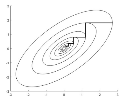
Conjugacy plays such an important role, because through it search directions can be constructed such that the new gradient $\mathbf{g}^{(k+1)}$ is not just orthogonal to the current search direction $\mathbf{d}^{(k)}$ but to all previous search directions. This avoids revisiting search directions as in Figure 2.1.
Specifically, the first search direction is chosen as $\mathbf{d}^{(0)}=-\mathbf{g}^{(0)}$. The following search directions are then constructed by
$$
\mathbf{d}^{(k)}=-\mathbf{g}^{(k)}+\beta^{(k)} \mathbf{d}^{(k-1)}, \quad k=1,2, \ldots,
$$
where $\beta^{(k)}$ is chosen such that the conjugacy condition $\mathbf{d}^{(k)^{T}} A \mathbf{d}^{(k-1)}=0$ is satisfied. This yields
$$
\beta^{(k)}=\frac{\mathbf{g}^{(k)^{T}} A \mathbf{d}^{(k-1)}}{\mathbf{d}^{(k-1)^{T}} A \mathbf{d}^{(k-1)}}, \quad k=1,2, \ldots
$$
This gives the conjugate gradient method.
The values of $\mathbf{x}^{(k+1)}$ and $\omega^{(k)}$ are calculated as before in (2.7) and $(2.9)$.
These search directions satisfy the descent condition. From Equation (2.8) we have seen that the descent condition is equivalent to $\mathbf{d}^{(k)^{T}} \mathbf{g}^{(k)}<0$. Using the formula for $\mathbf{d}^{(k)}$ above and the fact that the new gradient is orthogonal to the previous search direction, i.e., $\mathbf{d}^{(k-1)^{T}} \mathbf{g}^{(k)}=0$, we see that
$$
\mathbf{d}^{(k)^{T}} \mathbf{g}^{(k)}=-\left|\mathbf{g}^{(k)}\right|^{2}<0
$$
统计代写|数值分析和优化代写numerical analysis and optimazation代考|Krylov Subspaces and Pre-Conditioning
Definition 2.9. Let $A$ be an $n \times n$ matrix, $\mathbf{b} \in \mathbb{R}^{n}$ a non-zero vector, then for a number $m$ the space spanned by $A^{j} \mathbf{b}, j=0, \ldots, m-1$ is the $m^{\text {th }}$ Krylov subspace of $\mathbb{R}^{n}$ and is denoted by $K_{m}(A, \mathbf{b})$.
In our analysis of the conjugate gradient method we saw that in the $k^{\text {th }}$ iteration the space spanned by the search directions $\mathbf{d}^{(j)}$ and the space spanned by the gradients $\mathbf{g}^{(j)}, j=0, \ldots, k$, are the same.
Lemma 2.3. The space spanned by $\mathbf{g}^{(j)}\left(\right.$ or $\left.\mathbf{d}^{(j)}\right), j=0, \ldots, k$, is the same as the $k+1^{\text {th }}$ Krylov subspace.
Proof. For $k=0$ we have $\mathbf{d}^{(0)}=-\mathbf{g}^{(0)}=\mathbf{b} \in K_{1}(A, \mathbf{b})$.
We assume that the space spanned by $\mathbf{g}^{(j)}, j=0, \ldots, k$, is the same as the space spanned by $\mathbf{b}, A \mathbf{b}, \ldots, A^{k} \mathbf{b}$ and increase $k$ by one.
In the formula $\mathbf{g}^{(k+1)}=\mathbf{g}^{(k)}+\omega^{(k)} A \mathbf{d}^{(k)}$ both $\mathbf{g}^{(k)}$ and $\mathbf{d}^{(k)}$ can be expressed as linear combinations of $\mathbf{b}, A \mathbf{b}, \ldots, A^{k} \mathbf{b}$ by the inductive hypothesis. Thus $\mathbf{g}^{(k+1)}$ can be expressed as a linear combination of $\mathbf{b}, A \mathbf{b}, \ldots, A^{k+1} \mathbf{b}$. Equally, using $\mathbf{d}^{(k+1)}=-\mathbf{g}^{(k+1)}+\beta^{(k)} \mathbf{d}^{(k)}$ we show that $\mathbf{d}^{(k+1)}$ lies in the space spanned by b, $A \mathbf{b}, \ldots, A^{k+1} \mathbf{b}$, which is $K_{k+2}(A, \mathbf{b})$. This completes the proof.
In the following lemma we show some properties of the Krylov subspaces.
Lemma 2.4. Given $A$ and b. Then $K_{m}(A, \mathbf{b})$ is a subspace of $K_{m+1}(A, \mathbf{b})$ and there exists a positive integer $s \leq n$ such that for every $m \geq s K_{m}(A, \mathbf{b})=$ $K_{s}(A, \mathbf{b})$. Furthermore, if we express $\mathbf{b}$ as $\mathbf{b}=\sum_{i=1}^{t} c_{i} \mathbf{v}{i}$, where $\mathbf{v}{1}, \ldots, \mathbf{v}{t}$ are eigenvectors of $A$ corresponding to distinct eigenvalues and all coefficients $c{i}, i=1, \ldots, t$, are non-zero, then $s=t$.
Proof. Clearly, $K_{m}(A, \mathbf{b}) \subseteq K_{m+1}(A, \mathbf{b})$. The dimension of $K_{m}(A, \mathbf{b})$ is less than or equal to $m$, since it is spanned by $m$ vectors. It is also at most $n$ since
$K_{m}(A, \mathbf{b})$ is a subspace of $\mathbb{R}^{n}$. The first Krylov subspace has dimension 1 . We let $s$ be the greatest integer such that the dimension of $K_{s}(A, \mathbf{b})$ is $s$. Then the dimension of $K_{s+1}(A, \mathbf{b})$ cannot be $s+1$ by the choice of $s$. It has to be $s$, since $K_{s}(A, \mathbf{b}) \subseteq K_{s+1}(A, \mathbf{b})$. Hence the two spaces are the same. This means that $A^{s} \mathbf{b} \in K_{s}(A, \mathbf{b})$, i.e., $A^{s} \mathbf{b}=\sum_{j=0}^{s-1} a_{j} A^{j} \mathbf{b}$. But then
$$
A^{s+r} \mathbf{b}=\sum_{j=0}^{s-1} a_{j} A^{j+r} \mathbf{b}
$$
for any positive $r$. This means that also the spaces $K_{s+r+1}(A$, b $)$ and $K_{s+r}(A, \mathbf{b})$ are the same. Therefore, for every $m \geq s K_{m}(A, \mathbf{b})=K_{s}(A, \mathbf{b})$.
Suppose now that $\mathbf{b}=\sum_{i=1}^{t} c_{i} \mathbf{v}{i}$, where $\mathbf{v}{1}, \ldots, \mathbf{v}{t}$ are eigenvectors of $A$ corresponding to distinct eigenvalues $\lambda{i}$. Then for every $j=1, \ldots, s$
$$
A^{j} \mathbf{b}=\sum_{i=1}^{t} c_{i} \lambda_{i}^{j} \mathbf{v}_{i}
$$
统计代写|数值分析和优化代写numerical analysis and optimazation代考|Eigenvalues and Eigenvectors
So far we only considered eigenvalues when analyzing the properties of numerical methods. In the following sections we look at how to determine eigenvalues and eigenvectors. Let $A$ be a real $n \times n$ matrix. The eigenvalue equation is given by
$$
A \mathbf{v}=\lambda \mathbf{v} \text {, }
$$
where $\lambda$ is scalar. It may be complex if $A$ is not symmetric. There exists $\mathbf{v} \in \mathbb{R}^{n}$ satisfying the eigenvalue equation if and only if the determinant $\operatorname{det}(A-\lambda I)$ is zero. The function $p(\lambda)=\operatorname{det}(A-\lambda I), \lambda \in \mathbb{C}$, is a polynomial of degree $n$. However, calculating the eigenvalues by finding the roots of $p$ is generally unsuitable because of loss of accuracy due to rounding errors. In Chapter 1 , Fundamentals, we have seen how even finding the roots of a quadratic can be difficult due to loss of significance.
If the polynomial has some multiple roots and if $A$ is not symmetric, then $A$ might have less than $n$ linearly independent eigenvalues. However, there are always $n$ mutually orthogonal real eigenvectors when $A$ is symmetric. In the following we assume that $A$ has $n$ linearly independent eigenvectors $\mathbf{v}{j}$ for each eigenvalue $\lambda{j}, j=1, \ldots, n$. This can be achieved by perturbing $A$ slightly if necessary. The task is now to find $\mathbf{v}{j}$ and $\lambda{j}, j=1, \ldots, n$.
数值分析代写
统计代写|数值分析和优化代写numerical analysis and optimazation代考|Conjugate Gradients
We have already seen how the positive definiteness of A can be used to define a norm. This can be extended to have a concept similar to orthogonality.
Definition 2.8. The vectors u and v are conjugate with respect to the positive definite matrix A, if they are nonzero and satisfy uTAv=0.
Conjugacy plays such an important role, because through it search directions can be constructed such that the new gradient g(k+1) is not just orthogonal to the current search direction d(k) but to all previous search directions. This avoids revisiting search directions as in Figure 2.1.
Specifically, the first search direction is chosen as d(0)=−g(0). The following search directions are then constructed by
d(k)=−g(k)+β(k)d(k−1),k=1,2,…,
where β(k) is chosen such that the conjugacy condition d(k)TAd(k−1)=0 is satisfied. This yields
β(k)=g(k)TAd(k−1)d(k−1)TAd(k−1),k=1,2,…
This gives the conjugate gradient method.
The values of x(k+1) and ω(k) are calculated as before in (2.7) and (2.9).
These search directions satisfy the descent condition. From Equation (2.8) we have seen that the descent condition is equivalent to d(k)Tg(k)<0. Using the formula for d(k) above and the fact that the new gradient is orthogonal to the previous search direction, i.e., d(k−1)Tg(k)=0, we see that
d(k)Tg(k)=−|g(k)|2<0
统计代写|数值分析和优化代写numerical analysis and optimazation代考|Krylov Subspaces and Pre-Conditioning
Definition 2.9. Let A be an n×n matrix, b∈Rn a non-zero vector, then for a number m the space spanned by Ajb,j=0,…,m−1 is the mth Krylov subspace of Rn and is denoted by Km(A,b).
In our analysis of the conjugate gradient method we saw that in the kth iteration the space spanned by the search directions d(j) and the space spanned by the gradients g(j),j=0,…,k, are the same.
Lemma 2.3. The space spanned by g(j)( or d(j)),j=0,…,k, is the same as the k+1th Krylov subspace.
Proof. For k=0 we have d(0)=−g(0)=b∈K1(A,b).
We assume that the space spanned by g(j),j=0,…,k, is the same as the space spanned by b,Ab,…,Akb and increase k by one.
In the formula g(k+1)=g(k)+ω(k)Ad(k) both g(k) and d(k) can be expressed as linear combinations of b,Ab,…,Akb by the inductive hypothesis. Thus g(k+1) can be expressed as a linear combination of b,Ab,…,Ak+1b. Equally, using d(k+1)=−g(k+1)+β(k)d(k) we show that d(k+1) lies in the space spanned by b, Ab,…,Ak+1b, which is Kk+2(A,b). This completes the proof.
In the following lemma we show some properties of the Krylov subspaces.
Lemma 2.4. Given A and b. Then Km(A,b) is a subspace of Km+1(A,b) and there exists a positive integer s≤n such that for every m≥sKm(A,b)= Ks(A,b). Furthermore, if we express b as b=∑i=1tcivi, where v1,…,vt are eigenvectors of A corresponding to distinct eigenvalues and all coefficients ci,i=1,…,t, are non-zero, then s=t.
Proof. Clearly, Km(A,b)⊆Km+1(A,b). The dimension of Km(A,b) is less than or equal to m, since it is spanned by m vectors. It is also at most n since
Km(A,b) is a subspace of Rn. The first Krylov subspace has dimension 1 . We let s be the greatest integer such that the dimension of Ks(A,b) is s. Then the dimension of Ks+1(A,b) cannot be s+1 by the choice of s. It has to be s, since Ks(A,b)⊆Ks+1(A,b). Hence the two spaces are the same. This means that Asb∈Ks(A,b), i.e., Asb=∑j=0s−1ajAjb. But then
As+rb=∑j=0s−1ajAj+rb
for any positive r. This means that also the spaces Ks+r+1(A, b ) and Ks+r(A,b) are the same. Therefore, for every m≥sKm(A,b)=Ks(A,b).
Suppose now that b=∑i=1tcivi, where v1,…,vt are eigenvectors of A corresponding to distinct eigenvalues λi. Then for every j=1,…,s
Ajb=∑i=1tciλijvi
统计代写|数值分析和优化代写numerical analysis and optimazation代考|Eigenvalues and Eigenvectors
So far we only considered eigenvalues when analyzing the properties of numerical methods. In the following sections we look at how to determine eigenvalues and eigenvectors. Let A be a real n×n matrix. The eigenvalue equation is given by
Av=λv,
where λ is scalar. It may be complex if A is not symmetric. There exists v∈Rn satisfying the eigenvalue equation if and only if the determinant det(A−λI) is zero. The function p(λ)=det(A−λI),λ∈C, is a polynomial of degree n. However, calculating the eigenvalues by finding the roots of p is generally unsuitable because of loss of accuracy due to rounding errors. In Chapter 1 , Fundamentals, we have seen how even finding the roots of a quadratic can be difficult due to loss of significance.
If the polynomial has some multiple roots and if A is not symmetric, then A might have less than n linearly independent eigenvalues. However, there are always n mutually orthogonal real eigenvectors when A is symmetric. In the following we assume that A has n linearly independent eigenvectors vj for each eigenvalue λj,j=1,…,n. This can be achieved by perturbing A slightly if necessary. The task is now to find vj and λj,j=1,…,n.

统计代写请认准statistics-lab™. statistics-lab™为您的留学生涯保驾护航。统计代写|python代写代考
随机过程代考
在概率论概念中,随机过程是随机变量的集合。 若一随机系统的样本点是随机函数,则称此函数为样本函数,这一随机系统全部样本函数的集合是一个随机过程。 实际应用中,样本函数的一般定义在时间域或者空间域。 随机过程的实例如股票和汇率的波动、语音信号、视频信号、体温的变化,随机运动如布朗运动、随机徘徊等等。
贝叶斯方法代考
贝叶斯统计概念及数据分析表示使用概率陈述回答有关未知参数的研究问题以及统计范式。后验分布包括关于参数的先验分布,和基于观测数据提供关于参数的信息似然模型。根据选择的先验分布和似然模型,后验分布可以解析或近似,例如,马尔科夫链蒙特卡罗 (MCMC) 方法之一。贝叶斯统计概念及数据分析使用后验分布来形成模型参数的各种摘要,包括点估计,如后验平均值、中位数、百分位数和称为可信区间的区间估计。此外,所有关于模型参数的统计检验都可以表示为基于估计后验分布的概率报表。
广义线性模型代考
广义线性模型(GLM)归属统计学领域,是一种应用灵活的线性回归模型。该模型允许因变量的偏差分布有除了正态分布之外的其它分布。
statistics-lab作为专业的留学生服务机构,多年来已为美国、英国、加拿大、澳洲等留学热门地的学生提供专业的学术服务,包括但不限于Essay代写,Assignment代写,Dissertation代写,Report代写,小组作业代写,Proposal代写,Paper代写,Presentation代写,计算机作业代写,论文修改和润色,网课代做,exam代考等等。写作范围涵盖高中,本科,研究生等海外留学全阶段,辐射金融,经济学,会计学,审计学,管理学等全球99%专业科目。写作团队既有专业英语母语作者,也有海外名校硕博留学生,每位写作老师都拥有过硬的语言能力,专业的学科背景和学术写作经验。我们承诺100%原创,100%专业,100%准时,100%满意。
机器学习代写
随着AI的大潮到来,Machine Learning逐渐成为一个新的学习热点。同时与传统CS相比,Machine Learning在其他领域也有着广泛的应用,因此这门学科成为不仅折磨CS专业同学的“小恶魔”,也是折磨生物、化学、统计等其他学科留学生的“大魔王”。学习Machine learning的一大绊脚石在于使用语言众多,跨学科范围广,所以学习起来尤其困难。但是不管你在学习Machine Learning时遇到任何难题,StudyGate专业导师团队都能为你轻松解决。
多元统计分析代考
基础数据: $N$ 个样本, $P$ 个变量数的单样本,组成的横列的数据表
变量定性: 分类和顺序;变量定量:数值
数学公式的角度分为: 因变量与自变量
时间序列分析代写
随机过程,是依赖于参数的一组随机变量的全体,参数通常是时间。 随机变量是随机现象的数量表现,其时间序列是一组按照时间发生先后顺序进行排列的数据点序列。通常一组时间序列的时间间隔为一恒定值(如1秒,5分钟,12小时,7天,1年),因此时间序列可以作为离散时间数据进行分析处理。研究时间序列数据的意义在于现实中,往往需要研究某个事物其随时间发展变化的规律。这就需要通过研究该事物过去发展的历史记录,以得到其自身发展的规律。
回归分析代写
多元回归分析渐进(Multiple Regression Analysis Asymptotics)属于计量经济学领域,主要是一种数学上的统计分析方法,可以分析复杂情况下各影响因素的数学关系,在自然科学、社会和经济学等多个领域内应用广泛。
MATLAB代写
MATLAB 是一种用于技术计算的高性能语言。它将计算、可视化和编程集成在一个易于使用的环境中,其中问题和解决方案以熟悉的数学符号表示。典型用途包括:数学和计算算法开发建模、仿真和原型制作数据分析、探索和可视化科学和工程图形应用程序开发,包括图形用户界面构建MATLAB 是一个交互式系统,其基本数据元素是一个不需要维度的数组。这使您可以解决许多技术计算问题,尤其是那些具有矩阵和向量公式的问题,而只需用 C 或 Fortran 等标量非交互式语言编写程序所需的时间的一小部分。MATLAB 名称代表矩阵实验室。MATLAB 最初的编写目的是提供对由 LINPACK 和 EISPACK 项目开发的矩阵软件的轻松访问,这两个项目共同代表了矩阵计算软件的最新技术。MATLAB 经过多年的发展,得到了许多用户的投入。在大学环境中,它是数学、工程和科学入门和高级课程的标准教学工具。在工业领域,MATLAB 是高效研究、开发和分析的首选工具。MATLAB 具有一系列称为工具箱的特定于应用程序的解决方案。对于大多数 MATLAB 用户来说非常重要,工具箱允许您学习和应用专业技术。工具箱是 MATLAB 函数(M 文件)的综合集合,可扩展 MATLAB 环境以解决特定类别的问题。可用工具箱的领域包括信号处理、控制系统、神经网络、模糊逻辑、小波、仿真等。