如果你也在 怎样代写数据可视化Data visualization这个学科遇到相关的难题,请随时右上角联系我们的24/7代写客服。
数据可视化是将信息转化为视觉背景的做法,如地图或图表,使数据更容易被人脑理解并从中获得洞察力。数据可视化的主要目标是使其更容易在大型数据集中识别模式、趋势和异常值。
statistics-lab™ 为您的留学生涯保驾护航 在代写数据可视化Data visualization方面已经树立了自己的口碑, 保证靠谱, 高质且原创的统计Statistics代写服务。我们的专家在代写数据可视化Data visualization代写方面经验极为丰富,各种代写数据可视化Data visualization相关的作业也就用不着说。
我们提供的数据可视化Data visualization及其相关学科的代写,服务范围广, 其中包括但不限于:
- Statistical Inference 统计推断
- Statistical Computing 统计计算
- Advanced Probability Theory 高等概率论
- Advanced Mathematical Statistics 高等数理统计学
- (Generalized) Linear Models 广义线性模型
- Statistical Machine Learning 统计机器学习
- Longitudinal Data Analysis 纵向数据分析
- Foundations of Data Science 数据科学基础
统计代写|数据可视化代写Data visualization代考|Using Ggplot
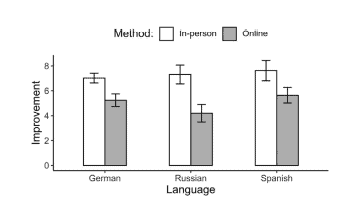
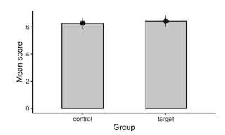
Recall that long is a dataset with ten participants, two groups (control and target), three tests, and test scores. A natural question to ask is whether the scores in both groups are different. ${ }^{21}$ For that, we could create a bar plot with scores on the $\gamma$-axis and the two groups on the $x$-axis. We want bars (which represent the mean for each group) as well as error bars (for standard errors)-see $₫ 1.3 .4$. An example is shown in Fig. 2.3.
You should look at any plot in $R$ as a collection of layers that are “stitched” together with a “+” sign. Each subsequent layer is automatically indented by RStudio and can add more information to a figure. The very first thing we need to do when using ggplot2 is to tell the package what data you need to plot. You can do that with the function ggplot(). Inside the function, we will also tell gaplot2 what we want to have on our axes. Let’s carefully go over the code that generates Fig. 2.3, shown in code block 9 .
In line 1 , we source our dataPrep. $R$ script (which itself will source other scripts). A month from now, we would simply open our R Project, click on our eda. $R$ script and, by running line 1 in code block 9 , all the tasks discussed earlier would be performed in the background. $R$ would import your data, load the necessary packages, and prepare the data, and we’d be ready to go. This automates the whole process of analyzing our data by splitting the task into separate scripts/components (which we created earlier). Chances are we won’t even remember what the previous tasks are a month from now, but we can always reopen those scripts and check them out.
统计代写|数据可视化代写Data visualization代考|Saving Your Plots
As with anything we do in $\mathrm{R}$, there are different ways to save your plot. However, before saving it, we should create a folder for it in our current directory (basics) -let’s call it figures. ${ }^{22}$ One way to save plots created with ggplot2 is to use the function ggsave() right after you run the code that generates your plot. Inside ggsave(), we specify the file name (and extension) that we wish to use (file), and we can also specify the scale of the figure as well as the DPI (dots per inch) for our figure (dpi). Thus, if you wanted to save the plot generated in code block 9 to the figures folder, you’d add a line of code after line 12 : ggsave (file = “figures/plot.jpg”, scale $=0.7, \mathrm{dpi}=$ “retina”). In this case, scale $=$ $0.7$ will generate a figure whose dimensions are $70 \%$ of what you can currently see in RStudio. Alternatively, you can manually specify the width and height of the figure by using the width and height arguments. To generate a plot with the exact same size as Fig. 2.3, use ggsave(file $=$ “figures/plot.jpg”, width $=4$, height $=2.5, \mathrm{dpi}=1000)^{23}$ If you realize the font size is too small in the figure, you can either change the dimensions in ggsave() (e.g., $3.5 \times 2$ instead of $4 \times 2.5$ will make the font look larger), or you can specify the
text size within ggplot()_an option we will explore later in the book (in chapter 5). In later chapters, code blocks that generate plots will have a ggsave() line, so you can easily save the plot.
As mentioned earlier, you can run the ggsave() line after running the lines that generate the actual plot (you may have already noticed that by pressing Cmd + Enter, RStudio will take you to the next line of code, so you can press Cmd + Enter again). Alternatively, you can select all the lines that generate the plot plus the line containing ggsave() and run all of them together. Either way, you will now have a file named plot.jpg in the figures directory (folder) of your R Project. ${ }^{24}$
To learn more about ggsave(), run ?ggsave()-the Help tab will show you the documentation for the function in pane D. Formats such as pdf or png are also accepted by ggsave()-check device in the documentation. We will discuss figures at length throughout the book, starting in $\$ 2.6 .2$.
Finally, you can also save a plot by clicking on Export in the Plots tab in pane D and then choosing whether you prefer to save it as an image or as a PDF file. This is a user-friendly way of saving your plot, but there are two caveats. First, the default dimensions of your figure may depend on your screen, so different people using your script may end up with a slightly different figure. Second, because this method involves clicking around, it’s not easily reproducible, since there are no lines of code in your script responsible for saving your figure.
统计代写|数据可视化代写Data visualization代考|General Guidelines for Data Visualization
There are at least two moments when visualizing data plays a key role in research. First, it helps us understand our own data. We typically need to see what’s going on with our data to decide what the best analysis is. Naturally, we can also use contingency tables and proportions/percentages, but more often than not figures will be the most appropriate way to do that. For example, if we want to verify whether our response variable is normally distributed, the quickest way to do that is to generate a simple histogram.
The second moment when visualizing data is crucial is when we communicate our findings in papers or at conferences. The effectiveness of a great idea can be compromised if it’s not communicated appropriately: if the reader (or the audience) cannot clearly see the patterns on which your analysis depends, your study may come across as less convincing or less meaningful. Furthermore, showing your data sends a message of transparency: if I can’t see your data or the patterns to which you refer, I might wonder why you’re not showing them to me.
These observations may seem obvious, but a great number of papers and presentations seem to ignore them. Overall, every study that uses data should show the patterns in the data. And because most studies in second language research rely on data, it wouldn’t be an exaggeration to assume that nearly all studies in the field should take data visualization seriously.
Now that you’ve seen a brief demonstration of how a figure can be generated in $\mathrm{R}$, let’s focus on some key conceptual aspects involving data visualization. Later, in chapters $3-5$, we will examine how to create figures in $\mathrm{R}$ in great detail.
数据可视化代考
统计代写|数据可视化代写Data visualization代考|Using Ggplot
回想一下,long 是一个包含十名参与者、两组(控制组和目标组)、三个测试和测试分数的数据集。一个自然要问的问题是两组的分数是否不同。21为此,我们可以创建一个带有分数的条形图C-轴和两组X-轴。我们想要条形图(代表每组的平均值)以及误差线形图(用于标准误差) – 见₫₫1.3.4. 示例如图 2.3 所示。
你应该看看任何情节R作为用“+”号“缝合”在一起的图层集合。每个后续层都由 RStudio 自动缩进,并且可以为图形添加更多信息。使用 ggplot2 时我们需要做的第一件事就是告诉包你需要绘制哪些数据。您可以使用函数 ggplot() 来做到这一点。在函数内部,我们还将告诉 gaplot2 我们想要在我们的轴上拥有什么。让我们仔细回顾一下生成图 2.3 的代码,如代码块 9 所示。
在第 1 行中,我们获取 dataPrep。R脚本(它本身将获取其他脚本)。一个月后,我们只需打开我们的 R 项目,点击我们的 eda。R脚本,并且通过在代码块 9 中运行第 1 行,前面讨论的所有任务都将在后台执行。R将导入您的数据,加载必要的包,并准备数据,我们就可以开始了。这通过将任务拆分为单独的脚本/组件(我们之前创建的)来自动化分析数据的整个过程。有可能我们甚至不记得一个月后以前的任务是什么,但我们总是可以重新打开这些脚本并检查它们。
统计代写|数据可视化代写Data visualization代考|Saving Your Plots
就像我们在R,有不同的方法来保存你的情节。但是,在保存它之前,我们应该在当前目录中为它创建一个文件夹(基础)——我们称之为图形。22保存使用 ggplot2 创建的绘图的一种方法是在运行生成绘图的代码后立即使用函数 ggsave()。在 ggsave() 中,我们指定了我们希望使用的文件名(和扩展名)(文件),我们还可以指定图形的比例以及图形的 DPI(每英寸点数)(dpi)。因此,如果您想将代码块 9 中生成的绘图保存到图形文件夹中,您需要在第 12 行之后添加一行代码:ggsave (file = “figures/plot.jpg”, scale=0.7,dp一世=“视网膜”)。在这种情况下,规模= 0.7将生成一个尺寸为70%您目前在 RStudio 中可以看到的内容。或者,您可以使用宽度和高度参数手动指定图形的宽度和高度。要生成与图 2.3 完全相同大小的图,请使用 ggsave(file=“figures/plot.jpg”,宽度=4, 高度=2.5,dp一世=1000)23如果您发现图中的字体太小,您可以在 ggsave() 中更改尺寸(例如,3.5×2代替4×2.5会使字体看起来更大),或者您可以指定
ggplot()_ 中的文本大小选项,我们将在本书后面(第 5 章)探讨。在后面的章节中,生成绘图的代码块将有一个 ggsave() 行,因此您可以轻松地保存绘图。
如前所述,您可以在运行生成实际绘图的行之后运行 ggsave() 行(您可能已经注意到,通过按 Cmd + Enter,RStudio 将带您进入下一行代码,因此您可以按 Cmd + 再次输入)。或者,您可以选择生成绘图的所有行以及包含 ggsave() 的行,然后将它们一起运行。无论哪种方式,您现在都将在 R 项目的图形目录(文件夹)中拥有一个名为 plot.jpg 的文件。24
要了解有关 ggsave() 的更多信息,请运行 ?ggsave() -“帮助”选项卡将在窗格 D 中显示该函数的文档。ggsave() 也接受 pdf 或 png 等格式 – 检查文档中的设备。我们将在整本书中详细讨论数字,从$2.6.2.
最后,您还可以通过单击窗格 D 中“绘图”选项卡中的“导出”来保存绘图,然后选择将其保存为图像还是 PDF 文件。这是保存情节的一种用户友好的方式,但有两个警告。首先,您的人物的默认尺寸可能取决于您的屏幕,因此使用您的脚本的不同人最终可能会得到略有不同的人物。其次,由于此方法涉及单击,因此不容易重现,因为脚本中没有负责保存图形的代码行。
统计代写|数据可视化代写Data visualization代考|General Guidelines for Data Visualization
至少有两个时刻可视化数据在研究中发挥关键作用。首先,它帮助我们理解我们自己的数据。我们通常需要查看我们的数据发生了什么来决定最好的分析是什么。当然,我们也可以使用列联表和比例/百分比,但通常情况下,数字是最合适的方法。例如,如果我们想验证我们的响应变量是否是正态分布的,那么最快的方法就是生成一个简单的直方图。
可视化数据至关重要的第二个时刻是当我们在论文或会议上交流我们的发现时。如果没有适当地传达一个好主意,它的有效性可能会受到影响:如果读者(或观众)无法清楚地看到您的分析所依赖的模式,您的研究可能会变得不那么令人信服或意义不大。此外,显示您的数据传递了一个透明的信息:如果我看不到您的数据或您所引用的模式,我可能想知道您为什么不向我显示它们。
这些观察结果似乎很明显,但大量论文和演讲似乎忽略了它们。总体而言,每项使用数据的研究都应显示数据中的模式。而且由于第二语言研究中的大多数研究都依赖于数据,因此可以毫不夸张地说,该领域的几乎所有研究都应该认真对待数据可视化。
现在您已经看到了如何生成图形的简短演示R,让我们关注一些涉及数据可视化的关键概念方面。后来,在章节3−5,我们将研究如何在R非常详细。

统计代写请认准statistics-lab™. statistics-lab™为您的留学生涯保驾护航。
金融工程代写
金融工程是使用数学技术来解决金融问题。金融工程使用计算机科学、统计学、经济学和应用数学领域的工具和知识来解决当前的金融问题,以及设计新的和创新的金融产品。
非参数统计代写
非参数统计指的是一种统计方法,其中不假设数据来自于由少数参数决定的规定模型;这种模型的例子包括正态分布模型和线性回归模型。
广义线性模型代考
广义线性模型(GLM)归属统计学领域,是一种应用灵活的线性回归模型。该模型允许因变量的偏差分布有除了正态分布之外的其它分布。
术语 广义线性模型(GLM)通常是指给定连续和/或分类预测因素的连续响应变量的常规线性回归模型。它包括多元线性回归,以及方差分析和方差分析(仅含固定效应)。
有限元方法代写
有限元方法(FEM)是一种流行的方法,用于数值解决工程和数学建模中出现的微分方程。典型的问题领域包括结构分析、传热、流体流动、质量运输和电磁势等传统领域。
有限元是一种通用的数值方法,用于解决两个或三个空间变量的偏微分方程(即一些边界值问题)。为了解决一个问题,有限元将一个大系统细分为更小、更简单的部分,称为有限元。这是通过在空间维度上的特定空间离散化来实现的,它是通过构建对象的网格来实现的:用于求解的数值域,它有有限数量的点。边界值问题的有限元方法表述最终导致一个代数方程组。该方法在域上对未知函数进行逼近。[1] 然后将模拟这些有限元的简单方程组合成一个更大的方程系统,以模拟整个问题。然后,有限元通过变化微积分使相关的误差函数最小化来逼近一个解决方案。
tatistics-lab作为专业的留学生服务机构,多年来已为美国、英国、加拿大、澳洲等留学热门地的学生提供专业的学术服务,包括但不限于Essay代写,Assignment代写,Dissertation代写,Report代写,小组作业代写,Proposal代写,Paper代写,Presentation代写,计算机作业代写,论文修改和润色,网课代做,exam代考等等。写作范围涵盖高中,本科,研究生等海外留学全阶段,辐射金融,经济学,会计学,审计学,管理学等全球99%专业科目。写作团队既有专业英语母语作者,也有海外名校硕博留学生,每位写作老师都拥有过硬的语言能力,专业的学科背景和学术写作经验。我们承诺100%原创,100%专业,100%准时,100%满意。
随机分析代写
随机微积分是数学的一个分支,对随机过程进行操作。它允许为随机过程的积分定义一个关于随机过程的一致的积分理论。这个领域是由日本数学家伊藤清在第二次世界大战期间创建并开始的。
时间序列分析代写
随机过程,是依赖于参数的一组随机变量的全体,参数通常是时间。 随机变量是随机现象的数量表现,其时间序列是一组按照时间发生先后顺序进行排列的数据点序列。通常一组时间序列的时间间隔为一恒定值(如1秒,5分钟,12小时,7天,1年),因此时间序列可以作为离散时间数据进行分析处理。研究时间序列数据的意义在于现实中,往往需要研究某个事物其随时间发展变化的规律。这就需要通过研究该事物过去发展的历史记录,以得到其自身发展的规律。
回归分析代写
多元回归分析渐进(Multiple Regression Analysis Asymptotics)属于计量经济学领域,主要是一种数学上的统计分析方法,可以分析复杂情况下各影响因素的数学关系,在自然科学、社会和经济学等多个领域内应用广泛。
MATLAB代写
MATLAB 是一种用于技术计算的高性能语言。它将计算、可视化和编程集成在一个易于使用的环境中,其中问题和解决方案以熟悉的数学符号表示。典型用途包括:数学和计算算法开发建模、仿真和原型制作数据分析、探索和可视化科学和工程图形应用程序开发,包括图形用户界面构建MATLAB 是一个交互式系统,其基本数据元素是一个不需要维度的数组。这使您可以解决许多技术计算问题,尤其是那些具有矩阵和向量公式的问题,而只需用 C 或 Fortran 等标量非交互式语言编写程序所需的时间的一小部分。MATLAB 名称代表矩阵实验室。MATLAB 最初的编写目的是提供对由 LINPACK 和 EISPACK 项目开发的矩阵软件的轻松访问,这两个项目共同代表了矩阵计算软件的最新技术。MATLAB 经过多年的发展,得到了许多用户的投入。在大学环境中,它是数学、工程和科学入门和高级课程的标准教学工具。在工业领域,MATLAB 是高效研究、开发和分析的首选工具。MATLAB 具有一系列称为工具箱的特定于应用程序的解决方案。对于大多数 MATLAB 用户来说非常重要,工具箱允许您学习和应用专业技术。工具箱是 MATLAB 函数(M 文件)的综合集合,可扩展 MATLAB 环境以解决特定类别的问题。可用工具箱的领域包括信号处理、控制系统、神经网络、模糊逻辑、小波、仿真等。