如果你也在 怎样代写数据科学data science这个学科遇到相关的难题,请随时右上角联系我们的24/7代写客服。
数据科学是一个跨学科领域,它使用科学方法、流程、算法和系统从嘈杂的、结构化和非结构化的数据中提取知识和见解,并在广泛的应用领域应用数据的知识和可操作的见解。
statistics-lab™ 为您的留学生涯保驾护航 在代写数据科学data science方面已经树立了自己的口碑, 保证靠谱, 高质且原创的统计Statistics代写服务。我们的专家在代写数据科学data science方面经验极为丰富,各种代写数据科学data science相关的作业也就用不着说。
我们提供的数据科学data science及其相关学科的代写,服务范围广, 其中包括但不限于:
- Statistical Inference 统计推断
- Statistical Computing 统计计算
- Advanced Probability Theory 高等楖率论
- Advanced Mathematical Statistics 高等数理统计学
- (Generalized) Linear Models 广义线性模型
- Statistical Machine Learning 统计机器学习
- Longitudinal Data Analysis 纵向数据分析
- Foundations of Data Science 数据科学基础
统计代写|数据科学代写data science代考|Algorithmic developments
Since the concept was proposed by Hastie and Stuetzle in 1989 , a considerable number of refinements and further developments have been reported. The first thrust of such developments address the issue of bias. The HSPCs algorithm has two biases, a model bias and an estimation bias.
Assuming that the data are subjected to some distribution function with gaussian noise, a model bias implies that that the radius of curvature in the curves is larger than the actual one. Conversely, spline functions applied by the algorithm results in an estimated radius that becomes smaller than the actual one.
With regards to the model bias, Tibshirani [69] assumed that data are generated in two stages (i) the points on the curve $f(t)$ are generated from some distribution function $\mu_{t}$ and (ii) $\mathbf{z}$ are formed based on conditional distribution $\mu_{z \mid t}$ (here the mean of $\mu_{z \mid t}$ is $\mathrm{f}(t)$ ). Assume that the distribution functions $\mu_{t}$
and $\mu_{z \mid t}$ are consistent with $\mu_{z}$, that is $\mu_{z}=\int \mu_{z \mid t}(\mathbf{z} \mid t) \mu_{t}(t) \mathrm{d} t$. Therefore, $\mathbf{z}$ are random vectors of dimension $N$ and subject to some density $\mu_{z}$. While the algorithm by Tibshirani [69] overcomes the model bias, the reported experimental results in this paper demonstrate that the practical improvement is marginal. Moreover, the self-consistent property is no longer valid.
In 1992 , Banfield and Raftery [4] addressed the estimation bias problem by replacing the squared distance error with residual and generalized the $\mathrm{PCs}$ into closed-shape curves. However, the refinement also introduces numerical instability and may form a smooth but otherwise incorrect principal curve.
In the mid 1990 s, Duchamp and Stuezle $[18,19]$ studied the holistical differential geometrical property of HSPCs, and analyzed the first and second variation of principal curves and the relationship between self-consistent and curvature of curves. This work discussed the existence of principal curves in the sphere, ellipse and annulus based on the geometrical characters of HSPCs. The work by Duchamp and Stuezle further proved that under the condition that curvature is not equal to zero, the expected square distance from data to principal curve in the plane is just a saddle point but not a local minimum unless low-frequency variation is considered to be described by a constraining term. As a result, cross-validation techniques can not be viewed as an effective measure to be used for the model selection of principal curves.
At the end of the 1990 s, Kégl proposed a new principal curve algorithm that incorporates a length constraint by combining vector quantization with principal curves. For this algorithm, further referred to as the $\mathrm{KPC}$ algorithm, Kégl proved that if and only if the data distribution has a finite secondorder moment, a KPC exists and is unique. This has been studied in detail based on the principle of structural risk minimization, estimation error and approximation error. It is proven in references $[34,35]$ that the $\mathrm{KPC}$ algorithm has a faster convergence rate that the other algorithms described above. This supports to use of the $\mathrm{KPC}$ algorithm for large databases.
统计代写|数据科学代写data science代考|Neural Network Approaches
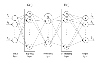
Using the structure shown in Fig. 1.6, Kramer [37] proposed an alternative NLPCA implementation to principal curves and manifolds. This structure represents an autoassociative neural network (ANN), which, in essence, is an identify mapping that consists of a total of 5 layers. Identify mapping relates to this hétwork topōlogy is optimized to reconstruct thẻ $N$ network input variables as accurately as possible using a reduced set of bottleneck nodes $n<N$. From the left to right, the first layer of the $\mathrm{ANN}$ is the input layer that passes weighted values of the original variable set $\mathbf{z}$ onto the second layer, that is the mapping layer:
$$
\xi_{i}=\sum_{j=1}^{N} w_{i j}^{(1)} z_{j}+b_{i}^{1}
$$
where $w_{i j}^{(1)}$ are the weights for the first layer and $b_{i}^{(1)}$ is a bias term. The sum in (1.41), $\xi_{i}$, is the input the the $i$ th node in the mapping layer that consists of a total of $M_{m}$ nodes. A scaled sum of the outputs of the nonlinearly transformed values $\sigma\left(\xi_{i}\right)$, then produce the nonlinear scores in the bottleneck layer. More precisely, the $p$ th nonlinear score $t_{p}, 1 \leq p \leq n$ is given by:
$$
t_{p}=\sum_{i=1}^{M_{m}} w_{p i}^{(2)} \sigma\left(\xi_{i}\right)+b_{p}^{(2)}=\sum_{i=1}^{M_{m}} w_{p i}^{(2)} \sigma\left(\sum_{j=1}^{N} w_{i j}^{(1)} z_{j}+b_{i}^{1}\right)+b_{p}^{(2)}
$$
To improve the modeling capability of the ANN structure for mildly nonlinear systems, it is useful to include linear contributions of the original variables $z_{1} z_{2} \cdots z_{N}$ :
$$
t_{p}=\sum_{i=1}^{M_{m}} w_{p i}^{(2)} \sigma\left(\sum_{j=1}^{N} w_{i j}^{(1)} z_{j}+b_{i}^{1}\right)+\sum_{j=1}^{N} w_{p i}^{(1 l)} z_{i}+b_{p}^{(2)}
$$
where the index $l$ refers to the linear contribution of the original variables. Such a network, where a direct linear contribution of the original variables is included, is often referred to as a generalized neural network. The middle layer of the ANN topology is further referred to as the bottleneck layer.
A linear combination of these nonlinear score variables then produces the inputs for the nodes in the 4 th layer, that is the demapping layer:
$$
\tau_{j}=\sum_{p=1}^{n} w_{j p}^{(3)} t_{p}+b_{p}^{(3)}
$$
Here, $w_{j p}^{(3)}$ and $b_{p}^{(3)}$ are the weights and the bias term associated with the bottleneck layer, respectively, that represents the input for the $j$ th node of the demapping layer. The nonlinear transformation of $\tau_{j}$ finally provides the reconstruction of the original variables $\mathbf{z}, \widehat{\mathbf{z}}=\left(\widehat{z}{1} \widehat{z}{2} \ldots \widehat{z}{N}\right)^{T}$ by the output layer: $$ \widehat{z}{q}=\sum_{j=1}^{M_{d}} w_{q j}^{(4)} \sigma\left(\sum_{p=1}^{n} w_{j p}^{(3)} t_{p}+b_{p}^{(3)}\right)+\sum_{j=1}^{n} w_{q j}^{(3 l)} t_{j}+b_{q}^{(4)}
$$
统计代写|数据科学代写data science代考|Introduction to kernel PCA
This technique first maps the original input vectors $\mathbf{z}$ onto a high-dimensional feature space $\mathbf{z} \mapsto \boldsymbol{\Phi}(\mathbf{z})$ and then perform the principal component analysis on $\Phi(\mathbf{z})$. Given a set of observations $\mathbf{z}{i} \in \mathbb{R}^{N}, i=\left{1 \quad 2 \cdots K^{*}\right}$, the mapping of $\mathbf{z}{i}$ onto a feature space, that is $\Phi(\mathbf{z})$ whose dimension is considerably larger than $N$, produces the following sample covarianee matrix:
$$
\mathbf{S}{\Phi \omega}=\frac{1}{K-1} \sum{i=1}^{K}\left(\boldsymbol{\Phi}\left(\mathbf{z}{i}\right)-\mathbf{m}{\Phi}\right)\left(\mathbf{\Phi}\left(\mathbf{z}{i}\right)-\mathbf{m}{\Phi}\right)^{T}=\frac{1}{K-1} \overline{\boldsymbol{\Phi}}(\mathbf{Z})^{T} \bar{\Phi}(\mathbf{Z}) .
$$
Here, $\mathrm{m}{\mathcal{s}}=\frac{1}{K} \Phi(\mathbf{Z})^{T} \mathbf{1}{K}$, where $\mathbf{1}{K} \in \mathbb{R}^{K}$ is a column vector storing unity elements, is the sample mean in the feature space, and $\Phi(\mathbf{Z})=$ $\left[\Phi\left(\mathbf{z}{1}\right) \Phi\left(\mathbf{z}{2}\right) \cdots \mathbf{\Phi}\left(\mathbf{z}{K}\right)\right]^{T}$ and $\bar{\Phi}(\mathbf{Z})=\Phi(\mathbf{Z})-\frac{1}{K} \mathbf{E}{K} \Phi(\mathbf{Z})$, with $\mathbf{E}{K}$ being a matrix of ones, are the original and mean centered feature matrices, respectively.
KPCA now solves the following eigenvector-eigenvalue problem,
$$
\mathbf{S}{\Phi \Phi} \mathbf{p}{i}=\frac{1}{K-1} \bar{\Phi}(\mathbf{Z})^{T} \overline{\boldsymbol{\Phi}}(\mathbf{Z}) \mathbf{p}{i}=\lambda{i} \mathbf{p}_{i} \quad i=1,2 \cdots N
$$ where $\lambda_{i}$ and $\mathbf{p}{i}$ are the eigenvalue and its associated eigenvector of $\mathbf{S}{\text {कw }}$. respectively. Given that the explicit mapping formulation of $\Phi(\mathbf{z})$ is usually unknown, it is difficult to extract the eigenvector-eigenvalue decomposition of $\mathbf{S}_{\Phi \Phi}$ directly. However, $\mathrm{KPCA}$ overcomes this deficiency as shown below.
数据可视化代写
统计代写|数据科学代写data science代考|Algorithmic developments
自从 Hastie 和 Stuetzle 于 1989 年提出这一概念以来,已经报道了相当多的改进和进一步的发展。这种发展的第一个重点是解决偏见问题。HSPCs 算法有两个偏差,一个模型偏差和一个估计偏差。
假设数据受到一些具有高斯噪声的分布函数的影响,模型偏差意味着曲线中的曲率半径大于实际的曲率半径。相反,算法应用的样条函数导致估计半径变得小于实际半径。
关于模型偏差,Tibshirani [69] 假设数据分两个阶段生成(i)曲线上的点F(吨)由一些分布函数生成μ吨(ii)和基于条件分布形成μ和∣吨(这里的意思是μ和∣吨是F(吨))。假设分布函数μ吨
和μ和∣吨与μ和, 那是μ和=∫μ和∣吨(和∣吨)μ吨(吨)d吨. 所以,和是维度的随机向量ñ并受到一定的密度μ和. 虽然 Tibshirani [69] 的算法克服了模型偏差,但本文报告的实验结果表明,实际改进是微不足道的。此外,自洽属性不再有效。
1992 年,Banfield 和 Raftery [4] 通过用残差代替平方距离误差解决了估计偏差问题,并推广了磷Cs成闭合曲线。然而,细化也引入了数值不稳定性,并可能形成平滑但不正确的主曲线。
1990 年代中期,Duchamp 和 Stuezle[18,19]研究了HSPCs的整体微分几何特性,分析了主曲线的一阶和二阶变化以及曲线自洽与曲率的关系。本工作基于HSPCs的几何特征,讨论了球面、椭圆和环面主曲线的存在。Duchamp 和 Stuezle 的工作进一步证明,在曲率不等于 0 的情况下,除非考虑低频变化,否则平面内数据到主曲线的期望平方距离只是鞍点而不是局部最小值用一个约束条件来描述。因此,交叉验证技术不能被视为主曲线模型选择的有效手段。
在 1990 年代末,Kégl 提出了一种新的主曲线算法,该算法通过将矢量量化与主曲线相结合来结合长度约束。对于该算法,进一步称为ķ磷CKégl 算法证明,当且仅当数据分布具有有限二阶矩时,KPC 存在并且是唯一的。这已经根据结构风险最小化、估计误差和近似误差的原理进行了详细的研究。已在参考文献中证明[34,35]那个ķ磷C算法具有比上述其他算法更快的收敛速度。这支持使用ķ磷C大型数据库的算法。
统计代写|数据科学代写data science代考|Neural Network Approaches
使用图 1.6 所示的结构,Kramer [37] 提出了一种替代主曲线和流形的 NLPCA 实现。这种结构代表了一个自关联神经网络(ANN),它本质上是一个识别映射,总共由 5 层组成。识别与此 hétwork 拓扑相关的映射被优化以重建 thẻñ使用减少的瓶颈节点集尽可能准确地网络输入变量n<ñ. 从左到右,第一层一种ññ是传递原始变量集的加权值的输入层和到第二层,即映射层:
X一世=∑j=1ñ在一世j(1)和j+b一世1
在哪里在一世j(1)是第一层的权重和b一世(1)是一个偏置项。(1.41) 中的总和,X一世, 是输入一世映射层中的第一个节点,总共由米米节点。非线性变换值的输出的缩放总和σ(X一世),然后在瓶颈层产生非线性分数。更准确地说,pth 非线性分数吨p,1≤p≤n是(谁)给的:吨p=∑一世=1米米在p一世(2)σ(X一世)+bp(2)=∑一世=1米米在p一世(2)σ(∑j=1ñ在一世j(1)和j+b一世1)+bp(2)
为了提高 ANN 结构对轻度非线性系统的建模能力,包括原始变量的线性贡献是有用的和1和2⋯和ñ :
吨p=∑一世=1米米在p一世(2)σ(∑j=1ñ在一世j(1)和j+b一世1)+∑j=1ñ在p一世(1l)和一世+bp(2)
索引在哪里l指原始变量的线性贡献。这种包含原始变量的直接线性贡献的网络通常被称为广义神经网络。ANN拓扑的中间层进一步称为瓶颈层。
这些非线性分数变量的线性组合然后为第 4 层(即去映射层)中的节点生成输入:
τj=∑p=1n在jp(3)吨p+bp(3)
这里,在jp(3)和bp(3)分别是与瓶颈层相关的权重和偏置项,表示j解映射层的第 th 节点。的非线性变换τj最后提供了原始变量的重建和,和^=(和^1和^2…和^ñ)吨通过输出层:和^q=∑j=1米d在qj(4)σ(∑p=1n在jp(3)吨p+bp(3))+∑j=1n在qj(3l)吨j+bq(4)
统计代写|数据科学代写data science代考|Introduction to kernel PCA
该技术首先映射原始输入向量和到高维特征空间和↦披(和)然后进行主成分分析披(和). 给定一组观察结果\mathbf{z}{i} \in \mathbb{R}^{N}, i=\left{1 \quad 2 \cdots K^{*}\right}\mathbf{z}{i} \in \mathbb{R}^{N}, i=\left{1 \quad 2 \cdots K^{*}\right}, 的映射和一世到特征空间上,即披(和)其尺寸远大于ñ,产生以下样本协变量矩阵:
小号披ω=1ķ−1∑一世=1ķ(披(和一世)−米披)(披(和一世)−米披)吨=1ķ−1披¯(从)吨披¯(从).
这里,米s=1ķ披(从)吨1ķ, 在哪里1ķ∈Rķ是存储单位元素的列向量,是特征空间中的样本均值,并且披(从)= [披(和1)披(和2)⋯披(和ķ)]吨和披¯(从)=披(从)−1ķ和ķ披(从), 和和ķ作为一个矩阵,分别是原始特征矩阵和均值中心特征矩阵。
KPCA 现在解决了以下特征向量-特征值问题,
小号披披p一世=1ķ−1披¯(从)吨披¯(从)p一世=λ一世p一世一世=1,2⋯ñ在哪里λ一世和p一世是特征值及其相关的特征向量क小号千瓦 . 分别。鉴于显式映射公式披(和)通常是未知的,很难提取特征向量-特征值分解小号披披直接地。然而,ķ磷C一种克服了这个不足,如下图所示。

统计代写请认准statistics-lab™. statistics-lab™为您的留学生涯保驾护航。统计代写|python代写代考
随机过程代考
在概率论概念中,随机过程是随机变量的集合。 若一随机系统的样本点是随机函数,则称此函数为样本函数,这一随机系统全部样本函数的集合是一个随机过程。 实际应用中,样本函数的一般定义在时间域或者空间域。 随机过程的实例如股票和汇率的波动、语音信号、视频信号、体温的变化,随机运动如布朗运动、随机徘徊等等。
贝叶斯方法代考
贝叶斯统计概念及数据分析表示使用概率陈述回答有关未知参数的研究问题以及统计范式。后验分布包括关于参数的先验分布,和基于观测数据提供关于参数的信息似然模型。根据选择的先验分布和似然模型,后验分布可以解析或近似,例如,马尔科夫链蒙特卡罗 (MCMC) 方法之一。贝叶斯统计概念及数据分析使用后验分布来形成模型参数的各种摘要,包括点估计,如后验平均值、中位数、百分位数和称为可信区间的区间估计。此外,所有关于模型参数的统计检验都可以表示为基于估计后验分布的概率报表。
广义线性模型代考
广义线性模型(GLM)归属统计学领域,是一种应用灵活的线性回归模型。该模型允许因变量的偏差分布有除了正态分布之外的其它分布。
statistics-lab作为专业的留学生服务机构,多年来已为美国、英国、加拿大、澳洲等留学热门地的学生提供专业的学术服务,包括但不限于Essay代写,Assignment代写,Dissertation代写,Report代写,小组作业代写,Proposal代写,Paper代写,Presentation代写,计算机作业代写,论文修改和润色,网课代做,exam代考等等。写作范围涵盖高中,本科,研究生等海外留学全阶段,辐射金融,经济学,会计学,审计学,管理学等全球99%专业科目。写作团队既有专业英语母语作者,也有海外名校硕博留学生,每位写作老师都拥有过硬的语言能力,专业的学科背景和学术写作经验。我们承诺100%原创,100%专业,100%准时,100%满意。
机器学习代写
随着AI的大潮到来,Machine Learning逐渐成为一个新的学习热点。同时与传统CS相比,Machine Learning在其他领域也有着广泛的应用,因此这门学科成为不仅折磨CS专业同学的“小恶魔”,也是折磨生物、化学、统计等其他学科留学生的“大魔王”。学习Machine learning的一大绊脚石在于使用语言众多,跨学科范围广,所以学习起来尤其困难。但是不管你在学习Machine Learning时遇到任何难题,StudyGate专业导师团队都能为你轻松解决。
多元统计分析代考
基础数据: $N$ 个样本, $P$ 个变量数的单样本,组成的横列的数据表
变量定性: 分类和顺序;变量定量:数值
数学公式的角度分为: 因变量与自变量
时间序列分析代写
随机过程,是依赖于参数的一组随机变量的全体,参数通常是时间。 随机变量是随机现象的数量表现,其时间序列是一组按照时间发生先后顺序进行排列的数据点序列。通常一组时间序列的时间间隔为一恒定值(如1秒,5分钟,12小时,7天,1年),因此时间序列可以作为离散时间数据进行分析处理。研究时间序列数据的意义在于现实中,往往需要研究某个事物其随时间发展变化的规律。这就需要通过研究该事物过去发展的历史记录,以得到其自身发展的规律。
回归分析代写
多元回归分析渐进(Multiple Regression Analysis Asymptotics)属于计量经济学领域,主要是一种数学上的统计分析方法,可以分析复杂情况下各影响因素的数学关系,在自然科学、社会和经济学等多个领域内应用广泛。
MATLAB代写
MATLAB 是一种用于技术计算的高性能语言。它将计算、可视化和编程集成在一个易于使用的环境中,其中问题和解决方案以熟悉的数学符号表示。典型用途包括:数学和计算算法开发建模、仿真和原型制作数据分析、探索和可视化科学和工程图形应用程序开发,包括图形用户界面构建MATLAB 是一个交互式系统,其基本数据元素是一个不需要维度的数组。这使您可以解决许多技术计算问题,尤其是那些具有矩阵和向量公式的问题,而只需用 C 或 Fortran 等标量非交互式语言编写程序所需的时间的一小部分。MATLAB 名称代表矩阵实验室。MATLAB 最初的编写目的是提供对由 LINPACK 和 EISPACK 项目开发的矩阵软件的轻松访问,这两个项目共同代表了矩阵计算软件的最新技术。MATLAB 经过多年的发展,得到了许多用户的投入。在大学环境中,它是数学、工程和科学入门和高级课程的标准教学工具。在工业领域,MATLAB 是高效研究、开发和分析的首选工具。MATLAB 具有一系列称为工具箱的特定于应用程序的解决方案。对于大多数 MATLAB 用户来说非常重要,工具箱允许您学习和应用专业技术。工具箱是 MATLAB 函数(M 文件)的综合集合,可扩展 MATLAB 环境以解决特定类别的问题。可用工具箱的领域包括信号处理、控制系统、神经网络、模糊逻辑、小波、仿真等。