如果你也在 怎样代写时间序列分析Time-Series Analysis这个学科遇到相关的难题,请随时右上角联系我们的24/7代写客服。
时间序列分析是分析在一个时间间隔内收集的一系列数据点的具体方式。在时间序列分析中,分析人员在设定的时间段内以一致的时间间隔记录数据点,而不仅仅是间歇性或随机地记录数据点。
statistics-lab™ 为您的留学生涯保驾护航 在代写时间序列分析Time-Series Analysis方面已经树立了自己的口碑, 保证靠谱, 高质且原创的统计Statistics代写服务。我们的专家在代写时间序列分析Time-Series Analysis代写方面经验极为丰富,各种代写时间序列分析Time-Series Analysis相关的作业也就用不着说。
我们提供的时间序列分析Time-Series Analysis及其相关学科的代写,服务范围广, 其中包括但不限于:
- Statistical Inference 统计推断
- Statistical Computing 统计计算
- Advanced Probability Theory 高等概率论
- Advanced Mathematical Statistics 高等数理统计学
- (Generalized) Linear Models 广义线性模型
- Statistical Machine Learning 统计机器学习
- Longitudinal Data Analysis 纵向数据分析
- Foundations of Data Science 数据科学基础
统计代写|时间序列分析代写Time-Series Analysis代考|Nonparametric Spectral Analysis
The nonparametric spectral analysis means that a spectral estimate is obtained directly from the time series without making any assumptions about its structure, except for its stationarity or, strictly speaking, its ergodicity. It can be obtained through a Fourier transform of the time series or of its parts with subsequent averaging and smoothing, through a Fourier transform of the covariance function estimate, or by applying a number of filters (windows, or tapers). Such methods are widely used in engineering, where the amount of data is often large and the experiments that generate data can often be repeated at will. The necessary software is easily available in R, MATLAB, and other packages for time series analysis. A thorough review of methods of spectral analysis with practical examples is given in Percival and Walden (1993). The traditional methods of nonparametric spectral analysis used in science and engineering include
- Blackman-Tukey method based upon the Fourier transform of the covariance function estimate plus some tapering (Blackman and Tukey 1958; Bendat and Piersol 1966),
- Bendat-Piersol method of nonoverlapping segments (Bendat and Piersol 2010),
- Welch’s overlapped segment averaging method (Welch 1967), and
- Thomson’s multitaper method (Thomson 1982).
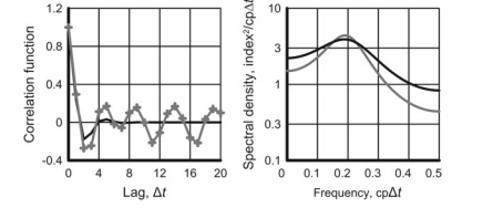
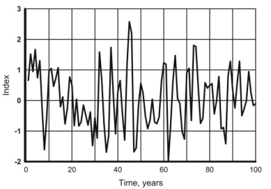
The first three methods are good for long time series and, with a few exceptions later in this chapter, they will rarely be applied here for analysis of time series, in particular, because so many of them are short. The fourth nonparametric method suggested by David Thomson, can produce, according to the author of the method as well as to this author’s experience, unbiased and consistent spectral estimates with short time series; it has high-frequency resolution and can be useful for detecting periodic and quasi-periodic components. In his original publication, the author of the method gave an example of successful analysis of a short $(N=100)$ time series with a rather complicated spectral density typical for sample records in communication systems. A brief explanation for the Thomson’s multitaper method (MTM) is that the spectral estimate is obtained as an average of several squared Fourier transforms of the time series which are smoothed with tapers (the so-called discrete prolate spheroidal sequences). This method of spectral analysis will be used in this book along with the autoregressive approach. A review of MTM can be found in Babadi and Brown (2014).
统计代写|时间序列分析代写Time-Series Analysis代考|Parametric Models of Time Series
The reliability problem with the nonparametric estimation of climate spectra exists due to the necessity to estimate many quantities in order to obtain a detailed and at the same time dependable estimate of the spectrum. When the Blackman-Tukey method is used, one needs to calculate the covariance function at many lags; otherwise, the spectral estimate will have low resolution in the frequency domain. And having many lags means poorer reliability. The Bendat and Piersol and Welch methods require splitting the original time series in as many shorter time series as possible and, at the same time, each subseries should be as long as possible. Therefore, even with a long time series, one has to find a compromise solution between the mutually contradicting desires to get a statistically reliable and, at the same time, high-resolution estimate. Obviously, this difficulty would have been less serious if the number of quantities to be estimated was small in comparison with the number of available observations. This improvement becomes possible with the parametric time series analysis.
The parametric approach arises mostly from the works of Yule (1927) and Wold (1938), who developed the concept of parametric models and introduced the general notion of a random process generated by a linear transformation of a white noise sequence-a linearly regular random process. In the autoregressive model, the current value of the process presents a linear combination of a finite number of its past values plus a “disturbance” consisting of the current value of the white noise sequence. Eventually, it gave rise to several types of parametric models, which are studied in detail in the classical book by Box and Jenkins (1970) and in its four subsequent editions. In this book, only the autoregressive models will be used as the means for obtaining parametric estimates of spectral density.
Though the spectral density function contains some information about the time series behavior in the time domain, it is the parametric approach, which allows one to obtain such information explicitly in the form of stochastic difference equations, with the simplest model being the white noise. In accordance with the definition given above, the time domain model of a stationary Markov chain is described with the following stochastic difference equation of order one:
$$
x_{t}=\varphi_{1} x_{t-1}+a_{t},
$$
统计代写|时间序列分析代写Time-Series Analysis代考|Parametric Spectral Analysis
The parametric approach to time series analysis allows one to obtain information about both time and frequency domain properties. By definition, the time series spectrum is the squared modulus of its Fourier transform: $s(f)=\left|\mathrm{FT}\left(x_{n}\right)\right|^{2}$. This way of spectrum estimation is inacceptable because the estimate is not efficient: its variance does not diminish as the time series length increases; however, it can be applied to the time series model, such as $\operatorname{AR}(p), \operatorname{MA}(q)$, or $\operatorname{ARMA}(p, q)$ given with Eqs. (3.4)-(3.6).
To obtain an equation for the spectral density through the autoregressive model, Eq. (3.4) can be rewritten as
$$
\left(1-\varphi_{1} B-\varphi_{2} B^{2}-\cdots-\varphi_{p} B^{p}\right) x_{t}=a_{t}
$$
The Fourier transform of this equation is obtained by substituting $\mathrm{e}^{-i 2 \pi j f \Delta t}$ for $B^{j}$ which leads to the following expression for the spectral density of an autoregressive process of order $p$ :
$$
s(f)=\frac{2 \sigma_{a}^{2} \Delta t}{\left|1-\sum_{j=1}^{p} \varphi_{j} \mathrm{e}^{-i 2 \pi j f \Delta t}\right|^{2}}, 0 \leq f \leq f_{N}
$$
where $i=\sqrt{-1}$. This equation means that, up to a multiplier, the spectral density of time series $x_{t}$ given with an autoregressive model $\operatorname{AR}(p)$ of order $p$ is defined with the autoregressive coefficients $\varphi_{j}, j=1, \ldots p$.
Applying the same technique to Eqs. (3.5) and (3.6) leads to the following expressions for spectral densities of the $\mathrm{MA}(q)$ and mixed $\operatorname{ARMA}(p, q)$ models of time series:
$$
s(f)=2 \sigma_{a}^{2} \Delta t\left|1-\sum_{j=1}^{q} \theta_{j} \mathrm{e}^{-i 2 \pi j f \Delta t}\right|^{2}
$$
and
$$
s(f)=\frac{2 \sigma_{a}^{2} \Delta t\left|1-\sum_{j=1}^{q} \theta_{j} \mathrm{e}^{-i 2 \pi j f \Delta t}\right|^{2}}{\left|1-\sum_{j=1}^{p} \varphi_{j} \mathrm{e}^{-i 2 \pi j f \Delta t}\right|^{2}}
$$
within the frequency range from 0 to $f_{N}$. Thus, the shape of the $\operatorname{ARMA}(p, q)$ spectrum is completely defined with $p+q$ parameters.
时间序列分析代考
统计代写|时间序列分析代写Time-Series Analysis代考|Nonparametric Spectral Analysis
非参数谱分析意味着谱估计是直接从时间序列中获得的,除了它的平稳性,或者严格地说,它的遍历性之外,不需要对其结构做任何假设。它可以通过时间序列或其部分的傅里叶变换以及随后的平均和平滑,通过协方差函数估计的傅里叶变换,或通过应用多个滤波器(窗口或锥形)来获得。这样的方法在工程中被广泛使用,其中数据量往往很大,产生数据的实验往往可以随意重复。必要的软件很容易在 R、MATLAB 和其他用于时间序列分析的软件包中获得。Percival 和 Walden (1993) 对光谱分析方法进行了全面的回顾,并给出了实际的例子。
- Blackman-Tukey 方法基于协方差函数估计的傅里叶变换加上一些锥度(Blackman 和 Tukey 1958;Bendat 和 Piersol 1966),
- 非重叠段的 Bendat-Piersol 方法(Bendat 和 Piersol 2010),
- Welch 的重叠分段平均方法 (Welch 1967),以及
- Thomson 的多锥度法(Thomson 1982)。
前三种方法适用于长时间序列,除了本章后面的少数例外,它们很少用于时间序列分析,特别是因为它们中的很多都是短的。根据该方法的作者以及作者的经验,David Thomson 提出的第四种非参数方法可以产生具有短时间序列的无偏和一致的谱估计;它具有高频分辨率,可用于检测周期性和准周期性分量。在他的原始出版物中,该方法的作者给出了一个成功分析一个简短的例子(ñ=100)具有相当复杂的频谱密度的时间序列,对于通信系统中的样本记录而言是典型的。对 Thomson 的多锥体方法 (MTM) 的简要解释是,光谱估计是作为时间序列的几个平方傅里叶变换的平均值获得的,这些变换用锥度进行平滑(所谓的离散长椭球体序列)。本书将使用这种光谱分析方法以及自回归方法。可以在 Babadi 和 Brown (2014) 中找到对 MTM 的评论。
统计代写|时间序列分析代写Time-Series Analysis代考|Parametric Models of Time Series
气候谱的非参数估计存在可靠性问题,因为需要估计许多量以获得详细且同时可靠的谱估计。当使用 Blackman-Tukey 方法时,需要计算许多滞后的协方差函数;否则,频谱估计将在频域中具有低分辨率。有很多滞后意味着更差的可靠性。Bendat、Piersol 和 Welch 方法要求将原始时间序列拆分为尽可能多的较短时间序列,同时每个子序列应尽可能长。因此,即使有很长的时间序列,也必须在相互矛盾的愿望之间找到一个折衷的解决方案,以获得统计上可靠的同时,高分辨率的估计。显然,如果要估计的数量与可用观测的数量相比较小,那么这个困难就不会那么严重。通过参数时间序列分析,这种改进成为可能。
参数方法主要源于 Yule (1927) 和 Wold (1938) 的工作,他们开发了参数模型的概念并引入了由白噪声序列的线性变换产生的随机过程的一般概念——线性规则随机过程。在自回归模型中,过程的当前值呈现有限数量的过去值加上由白噪声序列的当前值组成的“扰动”的线性组合。最终,它产生了几种类型的参数模型,在 Box 和 Jenkins(1970)的经典著作及其随后的四个版本中对其进行了详细研究。在本书中,只有自回归模型将用作获得谱密度参数估计的方法。
虽然谱密度函数包含一些关于时域中时间序列行为的信息,但它是参数化方法,它允许人们以随机差分方程的形式明确地获得这些信息,最简单的模型是白噪声。根据上面给出的定义,静止马尔可夫链的时域模型用以下一阶随机差分方程来描述:
X吨=披1X吨−1+一个吨,
统计代写|时间序列分析代写Time-Series Analysis代考|Parametric Spectral Analysis
时间序列分析的参数化方法允许人们获得有关时域和频域属性的信息。根据定义,时间序列谱是其傅里叶变换的平方模:s(F)=|F吨(Xn)|2. 这种频谱估计方式是不可接受的,因为估计效率不高:它的方差不会随着时间序列长度的增加而减小;但是,它可以应用于时间序列模型,例如和(p),嘛(q), 或者武器(p,q)用方程给出。(3.4)-(3.6)。
为了通过自回归模型获得谱密度方程,方程。(3.4) 可以改写为
(1−披1乙−披2乙2−⋯−披p乙p)X吨=一个吨
这个方程的傅里叶变换是通过代入得到的和−一世2圆周率jFΔ吨为了乙j这导致了自回归有序过程的谱密度的以下表达式p :
s(F)=2σ一个2Δ吨|1−∑j=1p披j和−一世2圆周率jFΔ吨|2,0≤F≤Fñ
在哪里一世=−1. 这个方程意味着,直到一个乘数,时间序列的谱密度X吨用自回归模型给出和(p)有秩序的p用自回归系数定义披j,j=1,…p.
将相同的技术应用于方程式。(3.5) 和 (3.6) 导致以下表达式的光谱密度米一个(q)并混合武器(p,q)时间序列模型:
s(F)=2σ一个2Δ吨|1−∑j=1qθj和−一世2圆周率jFΔ吨|2
和
s(F)=2σ一个2Δ吨|1−∑j=1qθj和−一世2圆周率jFΔ吨|2|1−∑j=1p披j和−一世2圆周率jFΔ吨|2
频率范围从 0 到Fñ. 因此,形状武器(p,q)频谱完全定义为p+q参数。

统计代写请认准statistics-lab™. statistics-lab™为您的留学生涯保驾护航。
金融工程代写
金融工程是使用数学技术来解决金融问题。金融工程使用计算机科学、统计学、经济学和应用数学领域的工具和知识来解决当前的金融问题,以及设计新的和创新的金融产品。
非参数统计代写
非参数统计指的是一种统计方法,其中不假设数据来自于由少数参数决定的规定模型;这种模型的例子包括正态分布模型和线性回归模型。
广义线性模型代考
广义线性模型(GLM)归属统计学领域,是一种应用灵活的线性回归模型。该模型允许因变量的偏差分布有除了正态分布之外的其它分布。
术语 广义线性模型(GLM)通常是指给定连续和/或分类预测因素的连续响应变量的常规线性回归模型。它包括多元线性回归,以及方差分析和方差分析(仅含固定效应)。
有限元方法代写
有限元方法(FEM)是一种流行的方法,用于数值解决工程和数学建模中出现的微分方程。典型的问题领域包括结构分析、传热、流体流动、质量运输和电磁势等传统领域。
有限元是一种通用的数值方法,用于解决两个或三个空间变量的偏微分方程(即一些边界值问题)。为了解决一个问题,有限元将一个大系统细分为更小、更简单的部分,称为有限元。这是通过在空间维度上的特定空间离散化来实现的,它是通过构建对象的网格来实现的:用于求解的数值域,它有有限数量的点。边界值问题的有限元方法表述最终导致一个代数方程组。该方法在域上对未知函数进行逼近。[1] 然后将模拟这些有限元的简单方程组合成一个更大的方程系统,以模拟整个问题。然后,有限元通过变化微积分使相关的误差函数最小化来逼近一个解决方案。
tatistics-lab作为专业的留学生服务机构,多年来已为美国、英国、加拿大、澳洲等留学热门地的学生提供专业的学术服务,包括但不限于Essay代写,Assignment代写,Dissertation代写,Report代写,小组作业代写,Proposal代写,Paper代写,Presentation代写,计算机作业代写,论文修改和润色,网课代做,exam代考等等。写作范围涵盖高中,本科,研究生等海外留学全阶段,辐射金融,经济学,会计学,审计学,管理学等全球99%专业科目。写作团队既有专业英语母语作者,也有海外名校硕博留学生,每位写作老师都拥有过硬的语言能力,专业的学科背景和学术写作经验。我们承诺100%原创,100%专业,100%准时,100%满意。
随机分析代写
随机微积分是数学的一个分支,对随机过程进行操作。它允许为随机过程的积分定义一个关于随机过程的一致的积分理论。这个领域是由日本数学家伊藤清在第二次世界大战期间创建并开始的。
时间序列分析代写
随机过程,是依赖于参数的一组随机变量的全体,参数通常是时间。 随机变量是随机现象的数量表现,其时间序列是一组按照时间发生先后顺序进行排列的数据点序列。通常一组时间序列的时间间隔为一恒定值(如1秒,5分钟,12小时,7天,1年),因此时间序列可以作为离散时间数据进行分析处理。研究时间序列数据的意义在于现实中,往往需要研究某个事物其随时间发展变化的规律。这就需要通过研究该事物过去发展的历史记录,以得到其自身发展的规律。
回归分析代写
多元回归分析渐进(Multiple Regression Analysis Asymptotics)属于计量经济学领域,主要是一种数学上的统计分析方法,可以分析复杂情况下各影响因素的数学关系,在自然科学、社会和经济学等多个领域内应用广泛。
MATLAB代写
MATLAB 是一种用于技术计算的高性能语言。它将计算、可视化和编程集成在一个易于使用的环境中,其中问题和解决方案以熟悉的数学符号表示。典型用途包括:数学和计算算法开发建模、仿真和原型制作数据分析、探索和可视化科学和工程图形应用程序开发,包括图形用户界面构建MATLAB 是一个交互式系统,其基本数据元素是一个不需要维度的数组。这使您可以解决许多技术计算问题,尤其是那些具有矩阵和向量公式的问题,而只需用 C 或 Fortran 等标量非交互式语言编写程序所需的时间的一小部分。MATLAB 名称代表矩阵实验室。MATLAB 最初的编写目的是提供对由 LINPACK 和 EISPACK 项目开发的矩阵软件的轻松访问,这两个项目共同代表了矩阵计算软件的最新技术。MATLAB 经过多年的发展,得到了许多用户的投入。在大学环境中,它是数学、工程和科学入门和高级课程的标准教学工具。在工业领域,MATLAB 是高效研究、开发和分析的首选工具。MATLAB 具有一系列称为工具箱的特定于应用程序的解决方案。对于大多数 MATLAB 用户来说非常重要,工具箱允许您学习和应用专业技术。工具箱是 MATLAB 函数(M 文件)的综合集合,可扩展 MATLAB 环境以解决特定类别的问题。可用工具箱的领域包括信号处理、控制系统、神经网络、模糊逻辑、小波、仿真等。