如果你也在 怎样代写机器学习machine learning这个学科遇到相关的难题,请随时右上角联系我们的24/7代写客服。
机器学习是对计算机算法的研究,这些算法可以通过经验和使用数据来自动改进。机器学习算法基于样本数据(称为训练数据)建立模型,以便在没有明确编程的情况下做出预测或决定。机器学习算法被广泛用于各种应用中,如医学、电子邮件过滤、语音识别和计算机视觉,在这些应用中,开发传统算法来执行所需的任务是困难的或不可行的。
statistics-lab™ 为您的留学生涯保驾护航 在代写机器学习machine learning方面已经树立了自己的口碑, 保证靠谱, 高质且原创的统计Statistics代写服务。我们的专家在代写机器学习machine learning代写方面经验极为丰富,各种代写机器学习machine learning相关的作业也就用不着说。
我们提供的机器学习machine learning及其相关学科的代写,服务范围广, 其中包括但不限于:
- Statistical Inference 统计推断
- Statistical Computing 统计计算
- Advanced Probability Theory 高等概率论
- Advanced Mathematical Statistics 高等数理统计学
- (Generalized) Linear Models 广义线性模型
- Statistical Machine Learning 统计机器学习
- Longitudinal Data Analysis 纵向数据分析
- Foundations of Data Science 数据科学基础
统计代写|机器学习代写machine learning代考|Leave-One-Out Machines
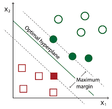
Theorem $2.37$ suggests an algorithm which directly minimizes the expression in the bound. The difficulty is that the resulting objective function will contain the step function $\mathbf{I}{t \geq 0}$. The idea we exploit is similar to the idea of soft margins in SVMs, where the step function is upper bounded by a piecewise linear function, also known as the hinge loss (see Figure 2.7). Hence, introducing slack variables, gives the following optimization problem: $$ \begin{array}{ll} \text { minimize } & \sum{i=1}^{m} \xi_{i} \
\text { subject to } \quad & y_{i} \sum_{\substack{j=1 \
j \neq i}}^{m} \alpha_{j} y_{j} k\left(x_{i}, x_{j}\right) \geq 1-\xi_{i} \quad i=1, \ldots, m, \
& \boldsymbol{\alpha} \geq \mathbf{0}, \boldsymbol{\xi} \geq \mathbf{0}
\end{array}
$$
For further classification of new test objects we use the decision rule given in equation (2.54). Let us study the resulting method which we call a leave-one-out machine (LOOM).
First, the technique appears to have no free regularization parameter. This should be compared with support vector machines, which control the amount of regularization through the free parameter $\lambda$. For SVMs, in the case of $\lambda \rightarrow 0$ one obtains a hard margin classifier with no training errors. In the case of linearly inseparable datasets in feature space (through noise, outliers or class overlap) one must admit some training errors (by constructing soft margins). To find the best choice of training error/margin tradeoff one must choose the appropriate value of $\lambda$. In leave-one-out machines a soft margin is automatically constructed. This happens because the algorithm does not attempt to minimize the number of training errors-it minimizes the number of training points that are classified incorrectly even when they are removed from the linear combination which forms the decision rule. However, if one can classify a training point correctly when it is removed from the linear combination, then it will always be classified correctly when it is placed back into the rule. This can be seen as $\alpha_{i} y_{i} k\left(x_{i}, x_{i}\right)$ always has the same sign as $y_{i}$; any training point is pushed further from the decision boundary by its own component of the linear combination. Note also that summing for all $j \neq i$ in the constraint $(2.56)$ is equivalent to setting the diagonal of the Gram matrix $\mathbf{G}$ to zero and instead summing for all $j$. Thus, the regularization employed by leave-one-out machines disregards the values $k\left(x_{i}, x_{i}\right)$ for all $i$.
Second, as for support vector machines, the solutions $\hat{\alpha} \in \mathbb{R}^{m}$ can be sparse in terms of the expansion vector; that is, only some of the coefficients $\hat{\alpha}_{i}$ are nonzero. As the coefficient of a training point does not contribute to its leave-one-out error in constraint (2.56), the algorithm does not assign a non-zero value to the coefficient of a training point in order to correctly classify it. A training point has to be classified correctly by the training points of the same label that are close to it, but the point itself makes no contribution to its own classification in training.
统计代写|机器学习代写machine learning代考|Pitfalls of Minimizing a Leave-One-Out Bound
The core idea of the presented algorithm is to directly minimize the leave-one-out bound. Thus, it seems that we are able to control the generalization ability of an algorithm disregarding quantities like the margin. This is not true in general ${ }^{18}$ and
in particular the presented algorithm is not able to achieve this goal. There are some pitfalls associated with minimizing a leave-one-out bound:
- In order to get a bound on the leave-one-out error we must specify the algorithm $\mathcal{A}$ beforehand. This is often done by specifying the form of the objective function which is to be maximized (or minimized) during learning. In our particular case we see that Theorem $2.37$ only considers algorithms defined by the maximization of $W$ ( $\alpha$ ) with the “box” constraint $0 \leq \boldsymbol{\alpha} \leq \mathbf{u}$. By changing the learning algorithm to minimize the bound itself we may well develop an optimization algorithm which is no longer compatible with the assumptions of the theorem. This is true in particular for leave-one-out machines which are no longer in the class of algorithms considered by Theorem $2.37$-whose bound they are aimed at minimizing. Further, instead of minimizing the bound directly we are using the hinge loss as anper bound on the Heaviside step function.
- The leave-one-out bound does not provide any guarantee about the generalization error $R[\mathcal{A}, z]$ (see Definition 2.10). Nonetheless, if the leave-one-out error is small then we know that, for most training samples $z \in \mathcal{Z}^{m}$, the resulting classifier has to have an expected risk close to that given by the bound. This is due to Hoeffding’s bound which says that for bounded loss (the expected risk of a hypothesis $f$ is bounded to the interval $[0,1])$ the expected risk $R[\mathcal{A}(z)]$ of the learned classifier $\mathcal{A}(z)$ is close to the expectation of the expected risk (bounded by the leave-one-out bound) with high probability over the random choice of the training sample. ${ }^{19}$ Note, however, that the leave-one-out estimate does not provide any information about the variance of the expected risk. Such information would allow the application of tighter bounds, for example, Chebyshev’s bound.
- The original motivation behind the use of the leave-one-out error was to measure the goodness of the hypothesis space $\mathcal{F}$ and of the learning algorithm $\mathcal{A}$ for the learning problem given by the unknown probability measure $\mathbf{P}{\mathbf{Z}}$. Commonly, the leave-one-out error is used to select among different models $\mathcal{F}{1}, \mathcal{F}_{2}, \ldots$ for a given learning algorithm $\mathcal{A}$. In this sense, minimizing the leave-one-out error is more a model selection strategy than a learning paradigm within a fixed model.
统计代写|机器学习代写machine learning代考|Adaptive Margin Machines
In order to generalize leave-one-out machines we see that the $m$ constraints in equation (2.56) can be rewritten as
$$
\begin{aligned}
y_{i} \sum_{\substack{j=1 \
j \neq i}}^{m} \alpha_{j} y_{j} k\left(x_{i}, x_{j}\right)+\alpha_{i} k\left(x_{i}, x_{i}\right) & \geq 1-\xi_{i}+\alpha_{i} k\left(x_{i}, x_{i}\right) \quad i=1, \ldots, m, \
y_{i} f\left(x_{i}\right) & \geq 1-\xi_{i}+\alpha_{i} k\left(x_{i}, x_{i}\right) \quad i=1, \ldots, m .
\end{aligned}
$$
Now, it is easy to see that a training point $\left(x_{i}, y_{i}\right) \in z$ is linearly penalized for failing to obtain a functional margin of $\bar{\gamma}{i}(\mathbf{w}) \geq 1+\alpha{i} k\left(x_{i}, x_{i}\right)$. In other words, the larger the contribution the training point makes to the decision rule (the larger the value of $\alpha_{i}$ ), the larger its functional margin must be. Thus, the algorithm controls the margin for each training point adaptively. From this formulation one can generalize the algorithm to control regularization through the margin loss. To make the margin at each training point a controlling variable we propose the following learning algorithm:
$$
\begin{array}{ll}
\text { minimize } & \sum_{i=1}^{m} \xi_{i} \
\text { subject to } \quad & y_{i} \sum_{j=1}^{m} \alpha_{j} y_{j} k\left(x_{i}, x_{j}\right) \geq 1-\xi_{i}+\lambda \alpha_{i} k\left(x_{i}, x_{i}\right), \quad i=1, \ldots, m . \
& \boldsymbol{\alpha} \geq \mathbf{0}, \xi \geq \mathbf{0}
\end{array}
$$ This algorithm-which we call adaptive margin machines-can also be viewed in the following way: If an object $x_{0} \in \boldsymbol{x}$ is an outlier (the kernel values w.r.t. points in its class are small and w.r.t. points in the other class are large), $\alpha_{o}$ in equation (2.58) must be large in order to classify $x_{o}$ correctly. Whilst support vector machines use the same functional margin of one for such an outlier, they attempt to classify $x_{o}$ correctly. In adaptive margin machines the functional margin is automatically increased to $1+\lambda \alpha_{o} k\left(x_{o}, x_{o}\right)$ for $x_{o}$ and thus less effort is made to change the decision function because each increase in $\alpha_{o}$ would lead to an even larger increase in $\xi_{o}$ and can therefore not be optimal.
机器学习代写
统计代写|机器学习代写machine learning代考|Leave-One-Out Machines
定理2.37提出了一种直接最小化边界表达式的算法。困难在于生成的目标函数将包含阶跃函数一世吨≥0. 我们利用的想法类似于 SVM 中的软边距的想法,其中阶跃函数的上限为分段线性函数,也称为铰链损失(见图 2.7)。因此,引入松弛变量,给出以下优化问题: 最小化 ∑一世=1米X一世 受制于 是一世∑j=1 j≠一世米一种j是jķ(X一世,Xj)≥1−X一世一世=1,…,米, 一种≥0,X≥0
为了进一步分类新的测试对象,我们使用方程(2.54)中给出的决策规则。让我们研究一下我们称之为留一法(LOOM)的方法。
首先,该技术似乎没有自由的正则化参数。这应该与支持向量机进行比较,支持向量机通过自由参数控制正则化量λ. 对于 SVM,在λ→0一个人获得了一个没有训练错误的硬边距分类器。对于特征空间中线性不可分的数据集(通过噪声、异常值或类重叠),必须承认一些训练错误(通过构建软边距)。为了找到训练误差/边际权衡的最佳选择,必须选择适当的值λ. 在留一法机器中,会自动构建软边距。发生这种情况是因为该算法并没有尝试最小化训练错误的数量——它最小化了错误分类的训练点的数量,即使它们从形成决策规则的线性组合中删除。但是,如果一个训练点在从线性组合中移除时可以正确分类,那么当它放回规则中时总是会正确分类。这可以看作一种一世是一世ķ(X一世,X一世)总是有相同的符号是一世; 任何训练点都被其自身的线性组合分量推离决策边界更远。另请注意,对所有人求和j≠一世在约束(2.56)相当于设置Gram矩阵的对角线G为零,而是对所有人求和j. 因此,留一法机器采用的正则化忽略了这些值ķ(X一世,X一世)对全部一世.
二、关于支持向量机,解一种^∈R米在扩展向量方面可以是稀疏的;也就是说,只有一些系数一种^一世是非零的。由于训练点的系数不会影响其在约束 (2.56) 中的留一错误,因此该算法不会为训练点的系数分配非零值以对其进行正确分类。一个训练点必须由与其接近的相同标签的训练点正确分类,但该点本身在训练中对其自身的分类没有任何贡献。
统计代写|机器学习代写machine learning代考|Pitfalls of Minimizing a Leave-One-Out Bound
所提出算法的核心思想是直接最小化留一出界。因此,我们似乎能够控制算法的泛化能力,而无需考虑诸如边际之类的量。一般情况下这是不正确的18和
特别是所提出的算法无法实现这一目标。有一些与最小化留一出界相关的陷阱:
- 为了得到留一错误的界限,我们必须指定算法一种预先。这通常通过指定在学习期间要最大化(或最小化)的目标函数的形式来完成。在我们的特殊情况下,我们看到定理2.37只考虑由最大化定义的算法在 ( 一种) 带有“盒子”约束0≤一种≤在. 通过改变学习算法以最小化界限本身,我们可以很好地开发一种不再与定理假设兼容的优化算法。对于不再属于 Theorem 所考虑的算法类别的留一法机器尤其如此2.37- 他们旨在最小化谁的界限。此外,我们不是直接最小化边界,而是使用铰链损失作为 Heaviside 阶跃函数的边界。
- 留一法不能保证泛化误差R[一种,和](见定义 2.10)。尽管如此,如果留一法误差很小,那么我们知道,对于大多数训练样本和∈从米,由此产生的分类器必须具有接近给定边界的预期风险。这是由于 Hoeffding 的界限,它表示对于有限损失(假设的预期风险F有界于区间[0,1])预期风险R[一种(和)]学习分类器的一种(和)在训练样本的随机选择上,以高概率接近预期风险的期望(以留一法为界)。19但是请注意,留一法估计不提供有关预期风险方差的任何信息。此类信息将允许应用更严格的界限,例如切比雪夫界限。
- 使用留一法误差的最初动机是衡量假设空间的优劣F和学习算法一种对于由未知概率测度给出的学习问题磷从. 通常,留一法误差用于在不同模型之间进行选择F1,F2,…对于给定的学习算法一种. 从这个意义上说,最小化留一法错误更像是一种模型选择策略,而不是固定模型中的学习范式。
统计代写|机器学习代写machine learning代考|Adaptive Margin Machines
为了概括留一法机器,我们看到米方程(2.56)中的约束可以重写为
是一世∑j=1 j≠一世米一种j是jķ(X一世,Xj)+一种一世ķ(X一世,X一世)≥1−X一世+一种一世ķ(X一世,X一世)一世=1,…,米, 是一世F(X一世)≥1−X一世+一种一世ķ(X一世,X一世)一世=1,…,米.
现在,很容易看出一个训练点(X一世,是一世)∈和因未能获得功能裕度而受到线性惩罚C¯一世(在)≥1+一种一世ķ(X一世,X一世). 也就是说,训练点对决策规则的贡献越大(一种一世),其功能余量必须越大。因此,该算法自适应地控制每个训练点的余量。从这个公式中,我们可以推广算法以通过边际损失控制正则化。为了使每个训练点的边距成为控制变量,我们提出了以下学习算法:
最小化 ∑一世=1米X一世 受制于 是一世∑j=1米一种j是jķ(X一世,Xj)≥1−X一世+λ一种一世ķ(X一世,X一世),一世=1,…,米. 一种≥0,X≥0这种算法——我们称之为自适应边距机——也可以用以下方式查看:如果一个对象X0∈X是一个异常值(其类中的内核值 wrt 点很小,而其他类中的 wrt 点很大),一种这等式 (2.58) 中的值必须很大才能分类X这正确。虽然支持向量机对这样的异常值使用相同的功能余量,但它们试图对X这正确。在自适应余量机器中,功能余量自动增加到1+λ一种这ķ(X这,X这)为了X这因此改变决策函数的努力会更少,因为每次增加一种这将导致更大的增长X这因此不可能是最优的。

统计代写请认准statistics-lab™. statistics-lab™为您的留学生涯保驾护航。
金融工程代写
金融工程是使用数学技术来解决金融问题。金融工程使用计算机科学、统计学、经济学和应用数学领域的工具和知识来解决当前的金融问题,以及设计新的和创新的金融产品。
非参数统计代写
非参数统计指的是一种统计方法,其中不假设数据来自于由少数参数决定的规定模型;这种模型的例子包括正态分布模型和线性回归模型。
广义线性模型代考
广义线性模型(GLM)归属统计学领域,是一种应用灵活的线性回归模型。该模型允许因变量的偏差分布有除了正态分布之外的其它分布。
术语 广义线性模型(GLM)通常是指给定连续和/或分类预测因素的连续响应变量的常规线性回归模型。它包括多元线性回归,以及方差分析和方差分析(仅含固定效应)。
有限元方法代写
有限元方法(FEM)是一种流行的方法,用于数值解决工程和数学建模中出现的微分方程。典型的问题领域包括结构分析、传热、流体流动、质量运输和电磁势等传统领域。
有限元是一种通用的数值方法,用于解决两个或三个空间变量的偏微分方程(即一些边界值问题)。为了解决一个问题,有限元将一个大系统细分为更小、更简单的部分,称为有限元。这是通过在空间维度上的特定空间离散化来实现的,它是通过构建对象的网格来实现的:用于求解的数值域,它有有限数量的点。边界值问题的有限元方法表述最终导致一个代数方程组。该方法在域上对未知函数进行逼近。[1] 然后将模拟这些有限元的简单方程组合成一个更大的方程系统,以模拟整个问题。然后,有限元通过变化微积分使相关的误差函数最小化来逼近一个解决方案。
tatistics-lab作为专业的留学生服务机构,多年来已为美国、英国、加拿大、澳洲等留学热门地的学生提供专业的学术服务,包括但不限于Essay代写,Assignment代写,Dissertation代写,Report代写,小组作业代写,Proposal代写,Paper代写,Presentation代写,计算机作业代写,论文修改和润色,网课代做,exam代考等等。写作范围涵盖高中,本科,研究生等海外留学全阶段,辐射金融,经济学,会计学,审计学,管理学等全球99%专业科目。写作团队既有专业英语母语作者,也有海外名校硕博留学生,每位写作老师都拥有过硬的语言能力,专业的学科背景和学术写作经验。我们承诺100%原创,100%专业,100%准时,100%满意。
随机分析代写
随机微积分是数学的一个分支,对随机过程进行操作。它允许为随机过程的积分定义一个关于随机过程的一致的积分理论。这个领域是由日本数学家伊藤清在第二次世界大战期间创建并开始的。
时间序列分析代写
随机过程,是依赖于参数的一组随机变量的全体,参数通常是时间。 随机变量是随机现象的数量表现,其时间序列是一组按照时间发生先后顺序进行排列的数据点序列。通常一组时间序列的时间间隔为一恒定值(如1秒,5分钟,12小时,7天,1年),因此时间序列可以作为离散时间数据进行分析处理。研究时间序列数据的意义在于现实中,往往需要研究某个事物其随时间发展变化的规律。这就需要通过研究该事物过去发展的历史记录,以得到其自身发展的规律。
回归分析代写
多元回归分析渐进(Multiple Regression Analysis Asymptotics)属于计量经济学领域,主要是一种数学上的统计分析方法,可以分析复杂情况下各影响因素的数学关系,在自然科学、社会和经济学等多个领域内应用广泛。
MATLAB代写
MATLAB 是一种用于技术计算的高性能语言。它将计算、可视化和编程集成在一个易于使用的环境中,其中问题和解决方案以熟悉的数学符号表示。典型用途包括:数学和计算算法开发建模、仿真和原型制作数据分析、探索和可视化科学和工程图形应用程序开发,包括图形用户界面构建MATLAB 是一个交互式系统,其基本数据元素是一个不需要维度的数组。这使您可以解决许多技术计算问题,尤其是那些具有矩阵和向量公式的问题,而只需用 C 或 Fortran 等标量非交互式语言编写程序所需的时间的一小部分。MATLAB 名称代表矩阵实验室。MATLAB 最初的编写目的是提供对由 LINPACK 和 EISPACK 项目开发的矩阵软件的轻松访问,这两个项目共同代表了矩阵计算软件的最新技术。MATLAB 经过多年的发展,得到了许多用户的投入。在大学环境中,它是数学、工程和科学入门和高级课程的标准教学工具。在工业领域,MATLAB 是高效研究、开发和分析的首选工具。MATLAB 具有一系列称为工具箱的特定于应用程序的解决方案。对于大多数 MATLAB 用户来说非常重要,工具箱允许您学习和应用专业技术。工具箱是 MATLAB 函数(M 文件)的综合集合,可扩展 MATLAB 环境以解决特定类别的问题。可用工具箱的领域包括信号处理、控制系统、神经网络、模糊逻辑、小波、仿真等。