如果你也在 怎样代写机器学习machine learning这个学科遇到相关的难题,请随时右上角联系我们的24/7代写客服。
机器学习是对计算机算法的研究,这些算法可以通过经验和使用数据来自动改进。机器学习算法基于样本数据(称为训练数据)建立模型,以便在没有明确编程的情况下做出预测或决定。机器学习算法被广泛用于各种应用中,如医学、电子邮件过滤、语音识别和计算机视觉,在这些应用中,开发传统算法来执行所需的任务是困难的或不可行的。
statistics-lab™ 为您的留学生涯保驾护航 在代写机器学习machine learning方面已经树立了自己的口碑, 保证靠谱, 高质且原创的统计Statistics代写服务。我们的专家在代写机器学习machine learning代写方面经验极为丰富,各种代写机器学习machine learning相关的作业也就用不着说。
我们提供的机器学习machine learning及其相关学科的代写,服务范围广, 其中包括但不限于:
- Statistical Inference 统计推断
- Statistical Computing 统计计算
- Advanced Probability Theory 高等概率论
- Advanced Mathematical Statistics 高等数理统计学
- (Generalized) Linear Models 广义线性模型
- Statistical Machine Learning 统计机器学习
- Longitudinal Data Analysis 纵向数据分析
- Foundations of Data Science 数据科学基础
统计代写|机器学习代写machine learning代考|Regularized Risk Functionals
One possible method of overcoming the lack of knowledge about $\mathbf{P}{\mathbf{Z}}$ is to replace it by its empirical estimate $\mathbf{v}{z}$. This principle, discussed in the previous section, justifies the perceptron learning algorithm. However, minimizing the empirical risk, as done by the perceptron learning algorithm, has several drawbacks:
- Many examples are required to ensure a small generalization error $R\left[\mathcal{A}_{\mathrm{ERM}}, z\right]$ with high probability taken over the random choice of $z$.
- There is no unique minimum, i.e., each weight vector $\mathbf{w} \in V(z)$ in version space parameterizes a classifier $f_{\mathrm{w}}$ that has $R_{\text {emp }}\left[f_{\mathrm{w}}, z\right]=0$.
- Without any further assumptions on $\mathbf{P}_{\mathbf{Z}}$ the number of steps until convergence of the perceptron learning algorithm is not bounded.
- A training sample $z \in Z^{m}$ that is linearly separable in feature space is required.
The second point in particular shows that ERM learning makes the learning task an ill-posed one (see Appendix A.4): A slight variation $\tilde{z}$ in the training sample $z$ might lead to a large deviation between the expected risks of the classifiers learned using the ERM principle, $\left|R\left[\mathcal{A}{\text {ERM }}(z)\right]-R\left[\mathcal{A}{\text {ERM }}(\tilde{z})\right]\right|$. As will be seen in Part II of this book, a very influential factor in this deviation is the possibility of the hypothesis space $\mathcal{F}$ adopting different labelings $\boldsymbol{y}$ for randomly drawn objects $\boldsymbol{x}$. The more diverse the set of functions a hypothesis space contains, the more easily
it can produce a given labeling $y$ regardless of how bad the subsequent prediction might be on new, as yet unseen, data points $z=(x, y)$. This effect is also known as overfitting, i.e., the empirical risk as given by equation (2.11) is much smaller than the expected risk ( $2.8$ ) we originally aimed at minimizing.
One way to overcome this problem is the method of regularization. In our example this amounts to introducing a regularizer a-priori, that is, a functional $\Omega: \mathcal{F} \rightarrow \mathbb{R}^{+}$, and defining the solution to the learning problem to be
$$
\mathcal{A}{\Omega}(z) \stackrel{\text { def }}{=} \underset{f \in \mathcal{F}}{\operatorname{argmin}} \underbrace{R{\mathrm{emp}}[f, z]+\lambda \Omega[f]}{R{\mathrm{reg}}[f, z]}
$$
统计代写|机器学习代写machine learning代考|Kernels and Linear Classifiers
As we assume $\phi$ to be given we will call this the explicit way to non-linearize a linear classification model. We already mentioned in Section $2.2$ that the number of dimensions, $n$, of the feature space has a great impact on the generalization ability of empirical risk minimization algorithms. Thus, one conceivable criterion for defining features $\phi_{i}$ is to seek a small set of basis functions $\phi_{i}$ which allow perfect discrimination between the classes in $\mathcal{X}$. This task is called feature selection.
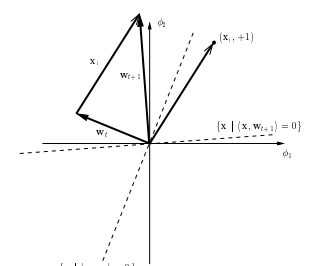
Let us return to the primal perceptron learning algorithm mentioned in the last subsection. As we start at $\mathbf{w}{0}=\mathbf{0}$ and add training examples only when a mistake is committed by the current hypothesis, it follows that the each solution has to admit a representation of the form, $$ \mathbf{w}{t}=\sum_{i=1}^{m} \alpha_{i} \phi\left(x_{i}\right)=\sum_{i=1}^{m} \alpha_{i} \mathbf{x}{i} $$ Hence, instead of formulating the perceptron algorithm in terms of the $n$ variables $\left(w{1}, \ldots, w_{n}\right)^{\prime}=\mathbf{w}$ we could learn the $m$ variables $\left(\alpha_{1}, \ldots, \alpha_{m}\right)^{\prime}=\alpha$ which we call the dual space of variables. In the case of perceptron learning we start with $\alpha_{0}=\mathbf{0}$ and then employ the representation of equation (2.17) to update $\boldsymbol{\alpha}{t}$ whenever a mistake occurs. To this end, we need to evaluate $$ y{j}\left\langle\mathbf{x}{j}, \mathbf{w}{t}\right\rangle=y_{j}\left\langle\mathbf{x}{j}, \sum{i=1}^{m} \alpha_{i} \mathbf{x}{i}\right\rangle=y{j} \sum_{i=1}^{m} \alpha_{i}\left\langle\mathbf{x}{j}, \mathbf{x}{i}\right\rangle
$$
which requires only knowledge of the inner product function $\langle\cdot, \cdot\rangle$ between the mapped training objects $\mathbf{x}$. Further, for the classification of a novel test object $x$ it suffices to know the solution vector $\alpha_{t}$ as well as the inner product function, because
$$
\left\langle\mathbf{x}, \mathbf{w}{t}\right\rangle=\left\langle\mathbf{x}, \sum{i=1}^{m} \alpha_{i} \mathbf{x}{i}\right\rangle=\sum{i=1}^{m} \alpha_{i}\left\langle\mathbf{x}, \mathbf{x}_{i}\right\rangle .
$$
统计代写|机器学习代写machine learning代考|The Kernel Technique
The key idea of the kernel technique is to invert the chain of arguments, i.e., choose a kernel $k$ rather than a mapping before applying a learning algorithm. Of course, not any symmetric function $k$ can serve as a kernel. The necessary and sufficient conditions of $k: \mathcal{X} \times \mathcal{X} \rightarrow \mathbb{R}$ to be a kernel are given by Mercer’s theorem. Before we rephrase the original theorem we give a more intuitive characterization of Mercer kernels.
Example 2.16 (Mercer’s theorem) Suppose our input space $\mathcal{X}$ has a finite number of elements, i.e., $\mathcal{X}=\left{x_{1}, \ldots, x_{r}\right}$. Then, the $r \times r$ kernel matrix $\mathbf{K}$ with $\mathbf{K}{i j}=k\left(x{i}, x_{j}\right)$ is by definition a symmetric matrix. Consider the eigenvalue decomposition of $\mathbf{K}=\mathbf{U} \mathbf{\Lambda} \mathbf{U}^{\prime}$, where $\mathbf{U}=\left(\mathbf{u}{1}^{\prime} ; \ldots ; \mathbf{u}{r}^{\prime}\right)$ is an $r \times n$ matrix such that $\mathbf{U}^{\prime} \mathbf{U}=\mathbf{I}{n}, \boldsymbol{\Lambda}=\operatorname{diag}\left(\lambda{1}, \ldots, \lambda_{n}\right), \lambda_{1} \geq \lambda_{2} \geq \cdots \geq \lambda_{n}>0$ and $n \leq r$ being known as the rank of the matrix $\mathbf{K}$ (see also Theorem A.83 and Definition A.62).
Now the mapping $\phi: \mathcal{X} \rightarrow \mathcal{K} \subseteq \ell_{2}^{n}$,
$\phi\left(x_{i}\right)=\boldsymbol{\Lambda}^{\frac{1}{2}} \mathbf{u}{i}$, leads to a Gram matrix $\mathbf{G}$ given by $$ \mathbf{G}{i j}=\left\langle\phi\left(x_{i}\right), \phi\left(x_{j}\right)\right\rangle_{\kappa}=\left(\boldsymbol{\Lambda}^{\frac{1}{2}} \mathbf{u}{i}\right)^{\prime}\left(\boldsymbol{\Lambda}^{\frac{1}{2}} \mathbf{u}{j}\right)=\mathbf{u}{i}^{\prime} \boldsymbol{\Lambda} \mathbf{u}{j}=\mathbf{K}{i j} . $$ We have constructed a feature space $\mathcal{K}$ and a mapping $\mathbf{\Lambda}$ into it purely from the kernel $k$. Note that $\lambda{n}>0$ is equivalent to assuming that $\mathbf{K}$ is positive semidefinite denoted by $\mathbf{K} \geq 0$ (see Definition A.40). In order to show that $\mathbf{K} \geq 0$ is also necessary for $k$ to be a kernel, we assume that $\lambda_{n}<0$. Then, the squared length of the nth mapped object $x_{n}$ is
$$
\left|\boldsymbol{\phi}\left(x_{n}\right)\right|^{2}=\mathbf{u}{n}^{\prime} \boldsymbol{\Lambda} \mathbf{u}{n}=\lambda_{n}<0,
$$
which contradicts the geometry in an inner product space.
Mercer’s theorem is an extension of this property, mainly achieved by studying the eigenvalue problem for integral equations of the form
$$
\int_{\mathcal{X}} k(x, \tilde{x}) f(\tilde{x}) d \tilde{x}=\lambda f(x),
$$
where $k$ is a bounded, symmetric and positive semidefinite function.
机器学习代写
统计代写|机器学习代写machine learning代考|Regularized Risk Functionals
一种可能的方法来克服缺乏知识磷从是用它的经验估计来代替它在和. 上一节中讨论的这一原则证明了感知器学习算法的合理性。然而,最小化经验风险,就像感知器学习算法所做的那样,有几个缺点:
- 需要许多示例来确保小的泛化错误R[一种和R米,和]以高概率接管随机选择和.
- 没有唯一的最小值,即每个权重向量在∈在(和)在版本空间中参数化分类器F在有R雇员 [F在,和]=0.
- 没有任何进一步的假设磷从直到感知器学习算法收敛的步数没有限制。
- 训练样本和∈从米需要在特征空间中线性可分。
第二点特别表明 ERM 学习使学习任务成为一个不适定的任务(见附录 A.4):略有不同和~在训练样本中和可能导致使用 ERM 原理学习的分类器的预期风险之间存在较大偏差,|R[一种风险管理 (和)]−R[一种风险管理 (和~)]|. 正如本书第二部分中将看到的,这种偏差的一个非常有影响的因素是假设空间的可能性F采用不同的标签是对于随机绘制的对象X. 假设空间包含的函数集越多样化,就越容易
它可以产生给定的标签是不管后续的预测对新的、尚未见过的数据点有多糟糕和=(X,是). 这种效应也称为过拟合,即方程(2.11)给出的经验风险远小于预期风险(2.8) 我们最初的目标是最小化。
克服这个问题的一种方法是正则化方法。在我们的示例中,这相当于引入了一个先验正则化器,即一个泛函Ω:F→R+,并将学习问题的解决方案定义为
一种Ω(和)= 定义 精氨酸F∈FR和米p[F,和]+λΩ[F]⏟Rr和G[F,和]
统计代写|机器学习代写machine learning代考|Kernels and Linear Classifiers
正如我们假设φ给出我们将其称为非线性化线性分类模型的显式方法。我们已经在章节中提到2.2维数,n, 特征空间的大小对经验风险最小化算法的泛化能力有很大影响。因此,定义特征的一个可以想象的标准φ一世是寻求一小组基函数φ一世这允许在类别之间进行完美区分X. 此任务称为特征选择。
让我们回到上一小节中提到的原始感知器学习算法。当我们开始在0=0并且仅当当前假设犯了错误时才添加训练示例,因此每个解决方案都必须承认形式的表示,在吨=∑一世=1米一种一世φ(X一世)=∑一世=1米一种一世X一世因此,不是根据n变量(在1,…,在n)′=在我们可以学习米变量(一种1,…,一种米)′=一种我们称之为变量的对偶空间。在感知器学习的情况下,我们从一种0=0然后使用方程(2.17)的表示来更新一种吨每当发生错误时。为此,我们需要评估是j⟨Xj,在吨⟩=是j⟨Xj,∑一世=1米一种一世X一世⟩=是j∑一世=1米一种一世⟨Xj,X一世⟩
只需要知道内积函数⟨⋅,⋅⟩映射的训练对象之间X. 此外,对于新测试对象的分类X知道解向量就足够了一种吨以及内积函数,因为
⟨X,在吨⟩=⟨X,∑一世=1米一种一世X一世⟩=∑一世=1米一种一世⟨X,X一世⟩.
统计代写|机器学习代写machine learning代考|The Kernel Technique
核技术的关键思想是反转参数链,即选择一个核ķ而不是应用学习算法之前的映射。当然,不是任何对称函数ķ可以作为内核。的充要条件ķ:X×X→R是由默瑟定理给出的内核。在我们重新表述原始定理之前,我们给出一个更直观的 Mercer 核表征。
例 2.16(默瑟定理)假设我们的输入空间X具有有限数量的元素,即\mathcal{X}=\left{x_{1}, \ldots, x_{r}\right}\mathcal{X}=\left{x_{1}, \ldots, x_{r}\right}. 然后,r×r核矩阵ķ和ķ一世j=ķ(X一世,Xj)根据定义,是一个对称矩阵。考虑特征值分解ķ=在Λ在′, 在哪里在=(在1′;…;在r′)是一个r×n矩阵使得在′在=一世n,Λ=诊断(λ1,…,λn),λ1≥λ2≥⋯≥λn>0和n≤r被称为矩阵的秩ķ(另见定理 A.83 和定义 A.62)。
现在映射φ:X→ķ⊆ℓ2n,
φ(X一世)=Λ12在一世, 导致一个 Gram 矩阵G由G一世j=⟨φ(X一世),φ(Xj)⟩ķ=(Λ12在一世)′(Λ12在j)=在一世′Λ在j=ķ一世j.我们构建了一个特征空间ķ和一个映射Λ纯粹从内核进入它ķ. 注意λn>0相当于假设ķ是半正定的,表示为ķ≥0(见定义 A.40)。为了表明ķ≥0也是必要的ķ作为一个内核,我们假设λn<0. 然后,第 n 个映射对象的平方长度Xn是
|φ(Xn)|2=在n′Λ在n=λn<0,
这与内积空间中的几何形状相矛盾。
Mercer 定理是这一性质的扩展,主要通过研究形式为的积分方程的特征值问题来实现
∫Xķ(X,X~)F(X~)dX~=λF(X),
在哪里ķ是有界、对称和半正定函数。

统计代写请认准statistics-lab™. statistics-lab™为您的留学生涯保驾护航。
金融工程代写
金融工程是使用数学技术来解决金融问题。金融工程使用计算机科学、统计学、经济学和应用数学领域的工具和知识来解决当前的金融问题,以及设计新的和创新的金融产品。
非参数统计代写
非参数统计指的是一种统计方法,其中不假设数据来自于由少数参数决定的规定模型;这种模型的例子包括正态分布模型和线性回归模型。
广义线性模型代考
广义线性模型(GLM)归属统计学领域,是一种应用灵活的线性回归模型。该模型允许因变量的偏差分布有除了正态分布之外的其它分布。
术语 广义线性模型(GLM)通常是指给定连续和/或分类预测因素的连续响应变量的常规线性回归模型。它包括多元线性回归,以及方差分析和方差分析(仅含固定效应)。
有限元方法代写
有限元方法(FEM)是一种流行的方法,用于数值解决工程和数学建模中出现的微分方程。典型的问题领域包括结构分析、传热、流体流动、质量运输和电磁势等传统领域。
有限元是一种通用的数值方法,用于解决两个或三个空间变量的偏微分方程(即一些边界值问题)。为了解决一个问题,有限元将一个大系统细分为更小、更简单的部分,称为有限元。这是通过在空间维度上的特定空间离散化来实现的,它是通过构建对象的网格来实现的:用于求解的数值域,它有有限数量的点。边界值问题的有限元方法表述最终导致一个代数方程组。该方法在域上对未知函数进行逼近。[1] 然后将模拟这些有限元的简单方程组合成一个更大的方程系统,以模拟整个问题。然后,有限元通过变化微积分使相关的误差函数最小化来逼近一个解决方案。
tatistics-lab作为专业的留学生服务机构,多年来已为美国、英国、加拿大、澳洲等留学热门地的学生提供专业的学术服务,包括但不限于Essay代写,Assignment代写,Dissertation代写,Report代写,小组作业代写,Proposal代写,Paper代写,Presentation代写,计算机作业代写,论文修改和润色,网课代做,exam代考等等。写作范围涵盖高中,本科,研究生等海外留学全阶段,辐射金融,经济学,会计学,审计学,管理学等全球99%专业科目。写作团队既有专业英语母语作者,也有海外名校硕博留学生,每位写作老师都拥有过硬的语言能力,专业的学科背景和学术写作经验。我们承诺100%原创,100%专业,100%准时,100%满意。
随机分析代写
随机微积分是数学的一个分支,对随机过程进行操作。它允许为随机过程的积分定义一个关于随机过程的一致的积分理论。这个领域是由日本数学家伊藤清在第二次世界大战期间创建并开始的。
时间序列分析代写
随机过程,是依赖于参数的一组随机变量的全体,参数通常是时间。 随机变量是随机现象的数量表现,其时间序列是一组按照时间发生先后顺序进行排列的数据点序列。通常一组时间序列的时间间隔为一恒定值(如1秒,5分钟,12小时,7天,1年),因此时间序列可以作为离散时间数据进行分析处理。研究时间序列数据的意义在于现实中,往往需要研究某个事物其随时间发展变化的规律。这就需要通过研究该事物过去发展的历史记录,以得到其自身发展的规律。
回归分析代写
多元回归分析渐进(Multiple Regression Analysis Asymptotics)属于计量经济学领域,主要是一种数学上的统计分析方法,可以分析复杂情况下各影响因素的数学关系,在自然科学、社会和经济学等多个领域内应用广泛。
MATLAB代写
MATLAB 是一种用于技术计算的高性能语言。它将计算、可视化和编程集成在一个易于使用的环境中,其中问题和解决方案以熟悉的数学符号表示。典型用途包括:数学和计算算法开发建模、仿真和原型制作数据分析、探索和可视化科学和工程图形应用程序开发,包括图形用户界面构建MATLAB 是一个交互式系统,其基本数据元素是一个不需要维度的数组。这使您可以解决许多技术计算问题,尤其是那些具有矩阵和向量公式的问题,而只需用 C 或 Fortran 等标量非交互式语言编写程序所需的时间的一小部分。MATLAB 名称代表矩阵实验室。MATLAB 最初的编写目的是提供对由 LINPACK 和 EISPACK 项目开发的矩阵软件的轻松访问,这两个项目共同代表了矩阵计算软件的最新技术。MATLAB 经过多年的发展,得到了许多用户的投入。在大学环境中,它是数学、工程和科学入门和高级课程的标准教学工具。在工业领域,MATLAB 是高效研究、开发和分析的首选工具。MATLAB 具有一系列称为工具箱的特定于应用程序的解决方案。对于大多数 MATLAB 用户来说非常重要,工具箱允许您学习和应用专业技术。工具箱是 MATLAB 函数(M 文件)的综合集合,可扩展 MATLAB 环境以解决特定类别的问题。可用工具箱的领域包括信号处理、控制系统、神经网络、模糊逻辑、小波、仿真等。