如果你也在 怎样代写机器学习machine learning这个学科遇到相关的难题,请随时右上角联系我们的24/7代写客服。
机器学习是一种数据分析的方法,可以自动建立分析模型。它是人工智能的一个分支,其基础是系统可以从数据中学习,识别模式,并在最小的人为干预下做出决定。
statistics-lab™ 为您的留学生涯保驾护航 在代写机器学习machine learning方面已经树立了自己的口碑, 保证靠谱, 高质且原创的统计Statistics代写服务。我们的专家在代写机器学习machine learning方面经验极为丰富,各种代写机器学习machine learning相关的作业也就用不着说。
我们提供的机器学习machine learning及其相关学科的代写,服务范围广, 其中包括但不限于:
- Statistical Inference 统计推断
- Statistical Computing 统计计算
- Advanced Probability Theory 高等楖率论
- Advanced Mathematical Statistics 高等数理统计学
- (Generalized) Linear Models 广义线性模型
- Statistical Machine Learning 统计机器学习
- Longitudinal Data Analysis 纵向数据分析
- Foundations of Data Science 数据科学基础
统计代写|机器学习作业代写machine learning代考|Performance Considerations
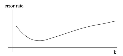
The $k-\mathrm{NN}$ technique is easy to implement in a computer program, and its behavior is easy to understand. But is there a reason to believe that its classification performance is good enough?
1-NN Versus Ideal Bayes The ultimate yardstick by which to assess any classifier’s success is the Bayesian formula. If the probabilities and $p d f$ ‘s employed in the Bayesian classifier are known with absolute accuracy, then this classifier-let us call it Ideal Bayes-exhibits the lowest error rate theoretically achievable on the given (noisy) data. It would be reassuring to realize that the $k$-NN paradigm does not trail too far behind.
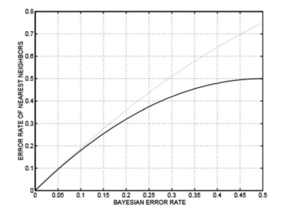
The question was subjected to rigorous mathematical analysis, and here are the results. Figure $3.4$ shows the comparison under such idealized circumstances as infinitely large training sets filling the instance space with infinite density. The solid curve represents the two-class case where each example is either positive or negative. We can see that if the error rate of Ideal Bayes is $5 \%$, the error rate of the 1-NN classifier (vertical axis) is $10 \%$. With the growing amount of noise, the difference between the two classifiers decreases, only to disappear when Ideal Bayes reaches $50 \%$ error rate – in which event, of course, the labels of the training examples are virtually random, and any attempt at automated classification is futile.
统计代写|机器学习作业代写machine learning代考|Weighted Nearest Neighbors
So far, the voting mechanism has been democratic in the sense that each nearest neighbor has the same vote. But while this seems appropriate, classification performance often improves if democracy is reduced.
Here is why. In Fig. 3.6, the task is to determine the class of object 1. Since three of the nearest neighbors are squares and only two circles, the 5 -NN classifier decides the object is square. However, a closer look reveals that the three square neighbors are quite distant from 1 , so much so that they perhaps should not have the same impact as the two circles in the object’s immediate vicinity. After all, we want to adhere to the requirement that $k$-NN should classify based on similarity-and more distant neighbors are less similar than closer ones.
Weighted Nearest Neighbors Domains of this kind motivate the introduction of weighted voting in which the weight of each neighbor depends on its distance from the object: the closer the neighbor, the greater its impact.
Let us denote the weights as $w_{1}, \ldots, w_{k}$. The weighted $k$ – $N N$ classifier sums up the weights of those neighbors that recommend the positive class (let the result be denoted by $\Sigma^{+}$) and then sums up the weights of those neighbors that support the negative class $\left(\Sigma^{-}\right)$. The final verdict depends on which is higher: if $\Sigma^{+}>\Sigma^{-}$, then the object is deemed positive; otherwise, it is labeled as negative. Generalization to domains with $n>2$ classes is straightforward.
For illustration, suppose the positive label is found in neighbors with weights $0.6$ and $0.7$, respectively, and the negative label is found in neighbors with weights $0.1,0.2$, and $0.3$. Weighted $k-\mathrm{NN}$ will choose the positive class because the combined weight of the positive neighbors, $\Sigma^{+}=0.6+0.7=1.3$, is greater than that of the negative neighbors, $\Sigma^{-}=0.1+0.2+0.3=0.6$. Just as in Fig. 3.6, the more frequent negative neighbors are outvoted by the less frequent positive neighbors because the latter are closer (and thus more similar) to the object we want to classify.
统计代写|机器学习作业代写machine learning代考|Removing Dangerous Examples
The value of each training example can be different. Some are typical of the classes they represent, others less so, and yet others may be downright misleading. This is why it is often a good thing to pre-process the training set: to remove examples suspected of not being useful.
The method of pre-processing is guided by the two observations illustrated in Fig. 3.7. First, an example labeled with one class but surrounded by examples of another class may indicate class-label noise. Second, examples from the borderline region separating two classes are unreliable: even small amount of noise in their attribute values can shift their locations in the wrong directions, thus affecting classification. Pre-processing seeks to remove these two types of examples from the training set.
机器学习代写
统计代写|机器学习作业代写machine learning代考|Performance Considerations
这ķ−ññ技术很容易在计算机程序中实现,其行为也很容易理解。但是有理由相信它的分类性能足够好吗?
1-NN 与理想贝叶斯 评估任何分类器成功与否的最终标准是贝叶斯公式。如果概率和pdF在贝叶斯分类器中使用的 ‘ 以绝对准确度为人所知,那么这个分类器——让我们称之为理想贝叶斯——表现出理论上在给定(嘈杂)数据上可实现的最低错误率。意识到ķ-NN 范式并没有落后太多。
这个问题经过了严格的数学分析,结果如下。数字3.4显示了在无限大的训练集以无限的密度填充实例空间的理想化情况下的比较。实线代表两类情况,其中每个例子要么是正面的,要么是负面的。我们可以看到,如果理想贝叶斯的错误率是5%,1-NN分类器的错误率(纵轴)为10%. 随着噪声量的增加,两个分类器之间的差异减小,直到理想贝叶斯达到50%错误率——当然,在这种情况下,训练样本的标签几乎是随机的,任何自动分类的尝试都是徒劳的。
统计代写|机器学习作业代写machine learning代考|Weighted Nearest Neighbors
到目前为止,投票机制是民主的,因为每个最近的邻居都有相同的投票。但是,虽然这似乎是合适的,但如果民主减少,分类性能通常会提高。
这就是为什么。在图 3.6 中,任务是确定对象 1 的类别。由于最近的三个邻居是正方形并且只有两个圆形,因此 5 -NN 分类器确定对象是正方形。然而,仔细观察会发现这三个正方形邻居与 1 相距甚远,以至于它们可能不应该与物体附近的两个圆圈产生相同的影响。毕竟,我们要遵守的要求是ķ-NN 应该基于相似性进行分类 – 更远的邻居比更近的邻居更不相似。
这种加权最近邻域激发了加权投票的引入,其中每个邻居的权重取决于其与对象的距离:邻居越近,其影响越大。
让我们将权重表示为在1,…,在ķ. 加权的ķ – ññ分类器将推荐正类的那些邻居的权重相加(让结果表示为Σ+) 然后将支持负类的那些邻居的权重相加(Σ−). 最终判决取决于哪个更高:如果Σ+>Σ−,则该对象被认为是积极的;否则,它被标记为负数。泛化到域n>2类很简单。
为了说明,假设在具有权重的邻居中找到正标签0.6和0.7,分别在具有权重的邻居中找到负标签0.1,0.2, 和0.3. 加权ķ−ññ将选择正类,因为正邻居的组合权重,Σ+=0.6+0.7=1.3, 大于负邻居的,Σ−=0.1+0.2+0.3=0.6. 就像在图 3.6 中一样,更频繁的负邻居被不频繁的正邻居投票,因为后者更接近(因此更相似)我们想要分类的对象。
统计代写|机器学习作业代写machine learning代考|Removing Dangerous Examples
每个训练示例的值可以不同。有些是他们所代表的阶级的典型,有些则不那么典型,还有一些可能是彻头彻尾的误导。这就是为什么对训练集进行预处理通常是一件好事:删除怀疑无用的示例。
预处理方法以图 3.7 中所示的两个观察结果为指导。首先,标有一个类但被另一类的示例包围的示例可能表示类标签噪声。其次,来自区分两个类别的边界区域的示例是不可靠的:即使它们的属性值中的少量噪声也会将它们的位置转移到错误的方向,从而影响分类。预处理旨在从训练集中删除这两种类型的示例。

统计代写请认准statistics-lab™. statistics-lab™为您的留学生涯保驾护航。统计代写|python代写代考
随机过程代考
在概率论概念中,随机过程是随机变量的集合。 若一随机系统的样本点是随机函数,则称此函数为样本函数,这一随机系统全部样本函数的集合是一个随机过程。 实际应用中,样本函数的一般定义在时间域或者空间域。 随机过程的实例如股票和汇率的波动、语音信号、视频信号、体温的变化,随机运动如布朗运动、随机徘徊等等。
贝叶斯方法代考
贝叶斯统计概念及数据分析表示使用概率陈述回答有关未知参数的研究问题以及统计范式。后验分布包括关于参数的先验分布,和基于观测数据提供关于参数的信息似然模型。根据选择的先验分布和似然模型,后验分布可以解析或近似,例如,马尔科夫链蒙特卡罗 (MCMC) 方法之一。贝叶斯统计概念及数据分析使用后验分布来形成模型参数的各种摘要,包括点估计,如后验平均值、中位数、百分位数和称为可信区间的区间估计。此外,所有关于模型参数的统计检验都可以表示为基于估计后验分布的概率报表。
广义线性模型代考
广义线性模型(GLM)归属统计学领域,是一种应用灵活的线性回归模型。该模型允许因变量的偏差分布有除了正态分布之外的其它分布。
statistics-lab作为专业的留学生服务机构,多年来已为美国、英国、加拿大、澳洲等留学热门地的学生提供专业的学术服务,包括但不限于Essay代写,Assignment代写,Dissertation代写,Report代写,小组作业代写,Proposal代写,Paper代写,Presentation代写,计算机作业代写,论文修改和润色,网课代做,exam代考等等。写作范围涵盖高中,本科,研究生等海外留学全阶段,辐射金融,经济学,会计学,审计学,管理学等全球99%专业科目。写作团队既有专业英语母语作者,也有海外名校硕博留学生,每位写作老师都拥有过硬的语言能力,专业的学科背景和学术写作经验。我们承诺100%原创,100%专业,100%准时,100%满意。
机器学习代写
随着AI的大潮到来,Machine Learning逐渐成为一个新的学习热点。同时与传统CS相比,Machine Learning在其他领域也有着广泛的应用,因此这门学科成为不仅折磨CS专业同学的“小恶魔”,也是折磨生物、化学、统计等其他学科留学生的“大魔王”。学习Machine learning的一大绊脚石在于使用语言众多,跨学科范围广,所以学习起来尤其困难。但是不管你在学习Machine Learning时遇到任何难题,StudyGate专业导师团队都能为你轻松解决。
多元统计分析代考
基础数据: $N$ 个样本, $P$ 个变量数的单样本,组成的横列的数据表
变量定性: 分类和顺序;变量定量:数值
数学公式的角度分为: 因变量与自变量
时间序列分析代写
随机过程,是依赖于参数的一组随机变量的全体,参数通常是时间。 随机变量是随机现象的数量表现,其时间序列是一组按照时间发生先后顺序进行排列的数据点序列。通常一组时间序列的时间间隔为一恒定值(如1秒,5分钟,12小时,7天,1年),因此时间序列可以作为离散时间数据进行分析处理。研究时间序列数据的意义在于现实中,往往需要研究某个事物其随时间发展变化的规律。这就需要通过研究该事物过去发展的历史记录,以得到其自身发展的规律。
回归分析代写
多元回归分析渐进(Multiple Regression Analysis Asymptotics)属于计量经济学领域,主要是一种数学上的统计分析方法,可以分析复杂情况下各影响因素的数学关系,在自然科学、社会和经济学等多个领域内应用广泛。
MATLAB代写
MATLAB 是一种用于技术计算的高性能语言。它将计算、可视化和编程集成在一个易于使用的环境中,其中问题和解决方案以熟悉的数学符号表示。典型用途包括:数学和计算算法开发建模、仿真和原型制作数据分析、探索和可视化科学和工程图形应用程序开发,包括图形用户界面构建MATLAB 是一个交互式系统,其基本数据元素是一个不需要维度的数组。这使您可以解决许多技术计算问题,尤其是那些具有矩阵和向量公式的问题,而只需用 C 或 Fortran 等标量非交互式语言编写程序所需的时间的一小部分。MATLAB 名称代表矩阵实验室。MATLAB 最初的编写目的是提供对由 LINPACK 和 EISPACK 项目开发的矩阵软件的轻松访问,这两个项目共同代表了矩阵计算软件的最新技术。MATLAB 经过多年的发展,得到了许多用户的投入。在大学环境中,它是数学、工程和科学入门和高级课程的标准教学工具。在工业领域,MATLAB 是高效研究、开发和分析的首选工具。MATLAB 具有一系列称为工具箱的特定于应用程序的解决方案。对于大多数 MATLAB 用户来说非常重要,工具箱允许您学习和应用专业技术。工具箱是 MATLAB 函数(M 文件)的综合集合,可扩展 MATLAB 环境以解决特定类别的问题。可用工具箱的领域包括信号处理、控制系统、神经网络、模糊逻辑、小波、仿真等。