如果你也在 怎样代写生物统计学Biostatistics这个学科遇到相关的难题,请随时右上角联系我们的24/7代写客服。
生物统计学是将统计技术应用于健康相关领域的科学研究,包括医学、生物学和公共卫生,并开发新的工具来研究这些领域。
statistics-lab™ 为您的留学生涯保驾护航 在代写生物统计学Biostatistics方面已经树立了自己的口碑, 保证靠谱, 高质且原创的统计Statistics代写服务。我们的专家在代写生物统计学Biostatistics方面经验极为丰富,各种代写生物统计学Biostatistics相关的作业也就用不着说。
我们提供的生物统计学Biostatistics及其相关学科的代写,服务范围广, 其中包括但不限于:
- Statistical Inference 统计推断
- Statistical Computing 统计计算
- Advanced Probability Theory 高等楖率论
- Advanced Mathematical Statistics 高等数理统计学
- (Generalized) Linear Models 广义线性模型
- Statistical Machine Learning 统计机器学习
- Longitudinal Data Analysis 纵向数据分析
- Foundations of Data Science 数据科学基础
统计代写|生物统计学作业代写Biostatistics代考|Shape of the Normal Curve
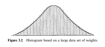
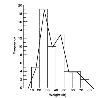
The histogram of Figure $2.3$ is reproduced here as Figure $3.1$ (for numerical details, see Table 2.2). A close examination shows that in general, the relative frequencies (or densities) are greatest in the vicinity of the intervals $20-29,30-$ 39 , and $40-49$ and decrease as we go toward both extremes of the range of measurements.Figure $3.1$ shows a distribution based on a total of 57 children; the frequency distribution consists of intervals with a width of $10 \mathrm{lb}$. Now imagine that we increase the number of children to 50,000 and decrease the width of the intervals to $0.01 \mathrm{lb}$. The histogram would now look more like the one in Figure $3.2$, where the step to go from one rectangular bar to the next is very small. Finally, suppose that we increase the number of children to 10 million and decrease the width of the interval to $0.00001 \mathrm{lb}$. You can now imagine a histogram with bars having practically no widths and thus the steps have all but disappeared. If we continue to increase the size of the data set and decrease the interval width, we eventually arrive at a smooth curve superimposed on the histogram of Figure $3.2$ called a density curve. You may already have heard about the normal distribution; it is described as being a bell-shaped distribution, sort of like a handlebar moustache, similar to Figure 3.2. The name may suggest that most dis-
tributions in nature are normal. Strictly speaking, that is false. Even more strictly speaking, they cannot be exactly normal. Some, such as heights of adults of a particular gender and race, are amazingly close to normal, but never exactly.
The normal distribution is extremely useful in statistics, but for a very different reason – not because it occurs in nature. Mathematicians proved that for samples that are “big enough,” values of their sample means, $\bar{x}^{\prime} s$ (including sample proportions as a special case), are approximately distributed as normal, even if the samples are taken from really strangely shaped distributions. This important result is called the central limit theorem. It is as important to statistics as the understanding of germs is to the understanding of disease. Keep in mind that “normal'” is just a name for this curve; if an attribute is not distributed normally, it does not imply that it is “abnormal.” Many statistics texts provide statistical procedures for finding out whether a distribution is normal, but they are beyond the scope of this book.
From now on, to distinguish samples from populations (a sample is a subgroup of a population), we adopt the set of notations defined in Table 3.7. Quantities in the second column $\left(\mu, \sigma^{2}\right.$, and $\pi$ ) are parameters representing numerical properties of populations; $\mu$ and $\sigma^{2}$ for continuously measured information and $\pi$ for binary information. Quantities in the first column $\left(\bar{x}, s^{2}\right.$, and $\left.p\right)$ are statistics representing summarized information from samples. Parameters are fixed (constants) but unknown, and each statistic can be used as an estimate for the parameter listed in the same row of the foregoing table. For example, $\bar{x}$ is used as an estimate of $\mu$; this topic is discussed in more detail in Chapter 4. A major problem in dealing with statistics such as $\bar{x}$ and $p$ is that if we take a different sample-even using the same sample size-values of a statistic change from sample to sample. The central limit theorem tells us that if sample sizes are fairly large, values of $\bar{x}$ (or $p$ ) in repeated sampling have a very nearly normal distribution. Therefore, to handle variability due to chance, so as to be able to declare-for example-that a certain observed difference is more than would occur by chance but is real, we first have to learn how to calculate probabilities associated with normal curves.
统计代写|生物统计学作业代写Biostatistics代考|Areas under the Standard Normal Curve
A variable that has a normal distribution with mean $\mu=0$ and variance $\sigma^{2}=1$ is called the standard normal variate and is commonly designated by the letter $Z$. As with any continuous variable, probability calculations here are always
concerned with finding the probability that the variable assumes any value in an interval between two specific points $a$ and $b$. The probability that a continuous variable assumes a value between two points $a$ and $b$ is the area under the graph of the density curve between $a$ and $b$; the vertical axis of the graph represents the densities as defined in Chapter 2. The total area under any such curve is unity (or $100 \%$ ), and Figure $3.4$ shows the standard normal curve with some important divisions. For example, about $68 \%$ of the area is contained within $\pm 1$ :
$$
\operatorname{Pr}(-1<z<1)=0.6826
$$
and about $95 \%$ within $\pm 2$ :
$$
\operatorname{Pr}(-2<z<2)=0.9545
$$
More areas under the standard normal curve have been computed and are available in tables, one of which is our Appendix B. The entries in the table of Appendix B give the area under the standard normal curve between the mean $(z=0)$ and a specified positive value of $z$. Graphically, it is represented by the shaded region in Figure 3.5.
Using the table of Appendix B and the symmetric property of the standard normal curve, we show how some other areas are computed. [With access to some computer packaged program, these can be obtained easily; see Section 3.5. However, we believe that these practices do add to the learning, even though they may no longer be needed.]
统计代写|生物统计学作业代写Biostatistics代考|Normal Distribution as a Probability Model
The reason we have been discussing the standard normal distribution so extensively with many examples is that probabilities for all normal distributions are computed using the standard normal distribution. That is, when we have a normal distribution with a given mean $\mu$ and a given standard deviation $\sigma$ (or
variance $\sigma^{2}$ ), we answer probability questions about the distribution by first converting (or standardizing) to the standard normal:
$$
z=\frac{x-\mu}{\sigma}
$$
Here we interpret the $z$ value (or $z$ score) as the number of standard deviations from the mean.
Example 3.7 If the total cholesterol values for a certain target population are approximately normally distributed with a mean of $200(\mathrm{mg} / 100 \mathrm{~mL})$ and a standard deviation of $20(\mathrm{mg} / 100 \mathrm{~mL}$ ), the probability that a person picked at random from this population will have a cholesterol value greater than $240(\mathrm{mg} / 100 \mathrm{~mL})$ is
$$
\begin{aligned}
\operatorname{Pr}(x \geq 240) &=\operatorname{Pr}\left(\frac{x-200}{20} \geq \frac{240-200}{20}\right) \
&=\operatorname{Pr}(z \geq 2.0) \
&=0.5-\operatorname{Pr}(z \leq 2.0) \
&=0.5-0.4772 \
&=0.0228 \text { or } 2.28 \%
\end{aligned}
$$
Example 3.8 Figure $3.11$ is a model for hypertension and hypotension (Journal of the American Medical Association, 1964), presented here as a simple illustration on the use of the normal distribution; acceptance of the model itself is not universal.
Data from a population of males were collected by age as shown in Table 3.9. From this table, using Appendix B, systolic blood pressure limits for each group can be calculated (Table $3.10$ ). For example, the highest healthy limit for the $20-24$ age group is obtained as follows.
生物统计代写
统计代写|生物统计学作业代写Biostatistics代考|Shape of the Normal Curve
图的直方图2.3此处转载为图3.1(有关数字的详细信息,请参见表 2.2)。仔细检查表明,一般而言,相对频率(或密度)在区间附近最大20−29,30−39 和40−49并且随着我们向测量范围的两个极端移动而减小。图3.1显示基于总共 57 个孩子的分布;频率分布由宽度为10lb. 现在想象我们将孩子的数量增加到 50,000 并将间隔的宽度减小到0.01lb. 直方图现在看起来更像图3.2,从一个矩形条到下一个矩形条的步长非常小。最后,假设我们将孩子的数量增加到 1000 万,并将区间的宽度减小到0.00001lb. 您现在可以想象一个直方图,其中条形几乎没有宽度,因此台阶几乎消失了。如果我们继续增加数据集的大小并减小区间宽度,我们最终会得到一条平滑的曲线叠加在图的直方图上3.2称为密度曲线。您可能已经听说过正态分布;它被描述为钟形分布,有点像车把胡子,类似于图 3.2。这个名字可能暗示大多数dis-
自然界的缘分是正常的。严格来说,这是错误的。更严格地说,它们不可能完全正常。有些,例如特定性别和种族的成年人的身高,惊人地接近正常值,但从未完全准确。
正态分布在统计学中非常有用,但出于一个非常不同的原因——不是因为它存在于自然界中。数学家证明,对于“足够大”的样本,它们的样本值意味着,X¯′s(包括作为特例的样本比例),即使样本是从非常奇怪形状的分布中获取的,也大致按正态分布。这个重要的结果被称为中心极限定理。对统计学的重要性就如同了解细菌对了解疾病一样重要。请记住,“正常”只是这条曲线的名称;如果一个属性不是正态分布的,并不意味着它是“异常的”。许多统计文本提供了用于确定分布是否正态的统计程序,但它们超出了本书的范围。
从现在开始,为了区分样本和总体(样本是总体的子组),我们采用表 3.7 中定义的一组符号。第二列中的数量(μ,σ2, 和圆周率) 是代表种群数值特性的参数;μ和σ2对于连续测量的信息和圆周率用于二进制信息。第一列中的数量(X¯,s2, 和p)是代表样本汇总信息的统计数据。参数是固定的(常数)但未知的,每个统计量都可以用作上表同一行中列出的参数的估计值。例如,X¯被用作估计μ; 第 4 章将更详细地讨论这个主题。处理统计数据的一个主要问题是X¯和p就是如果我们采用不同的样本——即使使用相同的样本量——样本之间的统计变化值。中心极限定理告诉我们,如果样本量相当大,则X¯(或者p) 在重复抽样中具有非常接近正态分布。因此,为了处理由偶然性引起的可变性,以便能够声明——例如——某个观察到的差异比偶然发生的要多,而是真实的,我们首先必须学习如何计算与正态曲线相关的概率。
统计代写|生物统计学作业代写Biostatistics代考|Areas under the Standard Normal Curve
具有均值正态分布的变量μ=0和方差σ2=1称为标准正态变量,通常用字母表示从. 与任何连续变量一样,这里的概率计算总是
关心找出变量在两个特定点之间的区间内取任何值的概率一种和b. 连续变量假设两点之间的值的概率一种和b是密度曲线图下的面积一种和b; 图表的纵轴代表第 2 章中定义的密度。任何此类曲线下的总面积为 1(或100%) 和图3.4显示带有一些重要部分的标准正态曲线。例如,关于68%该区域的包含在±1:
公关(−1<和<1)=0.6826
以及关于95%之内±2:
公关(−2<和<2)=0.9545
标准正态曲线下的更多面积已经计算出来,并在表格中提供,其中之一是我们的附录 B。附录 B 表格中的条目给出了平均值之间的标准正态曲线下面积(和=0)和一个指定的正值和. 在图形上,它由图 3.5 中的阴影区域表示。
使用附录 B 的表格和标准正态曲线的对称特性,我们展示了如何计算其他一些区域。【通过访问一些计算机打包程序,这些都可以很容易地获得;见第 3.5 节。然而,我们相信这些实践确实增加了学习,即使它们可能不再需要。]
统计代写|生物统计学作业代写Biostatistics代考|Normal Distribution as a Probability Model
我们用许多例子广泛讨论标准正态分布的原因是所有正态分布的概率都是使用标准正态分布计算的。也就是说,当我们有一个给定均值的正态分布时μ和给定的标准差σ(或者
方差σ2),我们通过首先转换(或标准化)为标准正态来回答有关分布的概率问题:
和=X−μσ
这里我们解读和值(或和分数)作为与平均值的标准偏差数。
例 3.7 如果某个目标人群的总胆固醇值近似正态分布,平均值为200(米G/100 米大号)和标准差20(米G/100 米大号),从该人群中随机挑选的人的胆固醇值大于240(米G/100 米大号)是
公关(X≥240)=公关(X−20020≥240−20020) =公关(和≥2.0) =0.5−公关(和≤2.0) =0.5−0.4772 =0.0228 或者 2.28%
示例 3.8 图3.11是高血压和低血压的模型(美国医学会杂志,1964 年),这里作为正态分布使用的简单说明;模型本身的接受度并不普遍。
来自男性群体的数据按年龄收集,如表 3.9 所示。根据该表,使用附录 B,可以计算每组的收缩压限值(表3.10)。例如,健康的最高限度20−24年龄组如下获得。

统计代写请认准statistics-lab™. statistics-lab™为您的留学生涯保驾护航。统计代写|python代写代考
随机过程代考
在概率论概念中,随机过程是随机变量的集合。 若一随机系统的样本点是随机函数,则称此函数为样本函数,这一随机系统全部样本函数的集合是一个随机过程。 实际应用中,样本函数的一般定义在时间域或者空间域。 随机过程的实例如股票和汇率的波动、语音信号、视频信号、体温的变化,随机运动如布朗运动、随机徘徊等等。
贝叶斯方法代考
贝叶斯统计概念及数据分析表示使用概率陈述回答有关未知参数的研究问题以及统计范式。后验分布包括关于参数的先验分布,和基于观测数据提供关于参数的信息似然模型。根据选择的先验分布和似然模型,后验分布可以解析或近似,例如,马尔科夫链蒙特卡罗 (MCMC) 方法之一。贝叶斯统计概念及数据分析使用后验分布来形成模型参数的各种摘要,包括点估计,如后验平均值、中位数、百分位数和称为可信区间的区间估计。此外,所有关于模型参数的统计检验都可以表示为基于估计后验分布的概率报表。
广义线性模型代考
广义线性模型(GLM)归属统计学领域,是一种应用灵活的线性回归模型。该模型允许因变量的偏差分布有除了正态分布之外的其它分布。
statistics-lab作为专业的留学生服务机构,多年来已为美国、英国、加拿大、澳洲等留学热门地的学生提供专业的学术服务,包括但不限于Essay代写,Assignment代写,Dissertation代写,Report代写,小组作业代写,Proposal代写,Paper代写,Presentation代写,计算机作业代写,论文修改和润色,网课代做,exam代考等等。写作范围涵盖高中,本科,研究生等海外留学全阶段,辐射金融,经济学,会计学,审计学,管理学等全球99%专业科目。写作团队既有专业英语母语作者,也有海外名校硕博留学生,每位写作老师都拥有过硬的语言能力,专业的学科背景和学术写作经验。我们承诺100%原创,100%专业,100%准时,100%满意。
机器学习代写
随着AI的大潮到来,Machine Learning逐渐成为一个新的学习热点。同时与传统CS相比,Machine Learning在其他领域也有着广泛的应用,因此这门学科成为不仅折磨CS专业同学的“小恶魔”,也是折磨生物、化学、统计等其他学科留学生的“大魔王”。学习Machine learning的一大绊脚石在于使用语言众多,跨学科范围广,所以学习起来尤其困难。但是不管你在学习Machine Learning时遇到任何难题,StudyGate专业导师团队都能为你轻松解决。
多元统计分析代考
基础数据: $N$ 个样本, $P$ 个变量数的单样本,组成的横列的数据表
变量定性: 分类和顺序;变量定量:数值
数学公式的角度分为: 因变量与自变量
时间序列分析代写
随机过程,是依赖于参数的一组随机变量的全体,参数通常是时间。 随机变量是随机现象的数量表现,其时间序列是一组按照时间发生先后顺序进行排列的数据点序列。通常一组时间序列的时间间隔为一恒定值(如1秒,5分钟,12小时,7天,1年),因此时间序列可以作为离散时间数据进行分析处理。研究时间序列数据的意义在于现实中,往往需要研究某个事物其随时间发展变化的规律。这就需要通过研究该事物过去发展的历史记录,以得到其自身发展的规律。
回归分析代写
多元回归分析渐进(Multiple Regression Analysis Asymptotics)属于计量经济学领域,主要是一种数学上的统计分析方法,可以分析复杂情况下各影响因素的数学关系,在自然科学、社会和经济学等多个领域内应用广泛。
MATLAB代写
MATLAB 是一种用于技术计算的高性能语言。它将计算、可视化和编程集成在一个易于使用的环境中,其中问题和解决方案以熟悉的数学符号表示。典型用途包括:数学和计算算法开发建模、仿真和原型制作数据分析、探索和可视化科学和工程图形应用程序开发,包括图形用户界面构建MATLAB 是一个交互式系统,其基本数据元素是一个不需要维度的数组。这使您可以解决许多技术计算问题,尤其是那些具有矩阵和向量公式的问题,而只需用 C 或 Fortran 等标量非交互式语言编写程序所需的时间的一小部分。MATLAB 名称代表矩阵实验室。MATLAB 最初的编写目的是提供对由 LINPACK 和 EISPACK 项目开发的矩阵软件的轻松访问,这两个项目共同代表了矩阵计算软件的最新技术。MATLAB 经过多年的发展,得到了许多用户的投入。在大学环境中,它是数学、工程和科学入门和高级课程的标准教学工具。在工业领域,MATLAB 是高效研究、开发和分析的首选工具。MATLAB 具有一系列称为工具箱的特定于应用程序的解决方案。对于大多数 MATLAB 用户来说非常重要,工具箱允许您学习和应用专业技术。工具箱是 MATLAB 函数(M 文件)的综合集合,可扩展 MATLAB 环境以解决特定类别的问题。可用工具箱的领域包括信号处理、控制系统、神经网络、模糊逻辑、小波、仿真等。