如果你也在 怎样代写贝叶斯分析Bayesian Analysis这个学科遇到相关的难题,请随时右上角联系我们的24/7代写客服。
贝叶斯分析,一种统计推断方法(以英国数学家托马斯-贝叶斯命名),允许人们将关于人口参数的先验信息与样本所含信息的证据相结合,以指导统计推断过程。
statistics-lab™ 为您的留学生涯保驾护航 在代写贝叶斯分析Bayesian Analysis方面已经树立了自己的口碑, 保证靠谱, 高质且原创的统计Statistics代写服务。我们的专家在代写贝叶斯分析Bayesian Analysis代写方面经验极为丰富,各种代写贝叶斯分析Bayesian Analysis相关的作业也就用不着说。
我们提供的贝叶斯分析Bayesian Analysis及其相关学科的代写,服务范围广, 其中包括但不限于:
- Statistical Inference 统计推断
- Statistical Computing 统计计算
- Advanced Probability Theory 高等概率论
- Advanced Mathematical Statistics 高等数理统计学
- (Generalized) Linear Models 广义线性模型
- Statistical Machine Learning 统计机器学习
- Longitudinal Data Analysis 纵向数据分析
- Foundations of Data Science 数据科学基础
统计代写|贝叶斯分析代写Bayesian Analysis代考|Bayesian point estimation
Once the posterior distribution or density $f(\theta \mid y)$ has been obtained, Bayesian point estimates of the model parameter $\theta$ can be calculated. The three most commonly used point estimates are as follows.
- The posterior mean of $\theta$ is
$$
E(\theta \mid y)=\int \theta d F(\theta \mid y)= \begin{cases}\int \theta f(\theta \mid y) d \theta & \text { if } \theta \text { is continuous } \ \sum_{\theta} \theta f(\theta \mid y) & \text { if } \theta \text { is discrete. }\end{cases}
$$ - The posterior mode of $\theta$ is
$\operatorname{Mode}(\theta \mid y)=$ any value $m \in \mathfrak{R}$ which satisfies
$$
f(\theta=m \mid x)=\max {\theta} f(\theta \mid x) $$ or $\lim {\theta \rightarrow m} f(\theta \mid x)=\sup f(\theta \mid x)$,
or the set of all such values. - The posterior median of $\theta$ is
$\operatorname{Median}(\theta \mid y)=$ any value $m$ of $\theta$ such that
$$
\begin{array}{r}
P(\theta \leq m \mid y) \geq 1 / 2 \
\text { and } P(\theta \geq m \mid y) \geq 1 / 2
\end{array}
$$
or the set of all such values.
统计代写|贝叶斯分析代写Bayesian Analysis代考|Bayesian interval estimation
There are many ways to construct a Bayesian interval estimate, but the two most common ways are defined as follows. The $1-\alpha$ (or $100(1-\alpha) \%$ ) highest posterior density region (HPDR) for $\theta$ is the smallest set $S$ such that:
$$
P(\theta \in S \mid y) \geq 1-\alpha
$$
and $f\left(\theta_{1} \mid y\right) \geq f\left(\theta_{2} \mid y\right)$ if $\theta_{1} \in S$ and $\theta_{2} \notin S$.
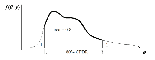
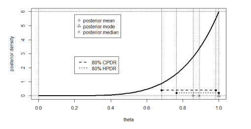
Figure $1.6$ illustrates the idea of the HPDR. In the very common situation where $\theta$ is scalar, continuous and has a posterior density which is unimodal with no local modes (i.e. has the form of a single ‘mound’), the 1- $\alpha$ HPDR takes on the form of a single interval defined by two points at which the posterior density has the same value. When the HPDR is a single interval, it is the shortest possible single interval over which the area under the posterior density is $1-\alpha$.
The $1-\alpha$ central posterior density region (CPDR) for a scalar parameter $\theta$ may be defined as the shortest single interval $[a, b]$ such that:
$P(\thetab \mid y) \leq \alpha / 2$.
In the common case of a continuous parameter with a posterior density in the form of a single ‘mound’ which is furthermore symmetric, the CPDR and HPDR are identical.
Note 1: The 1- $\alpha$ CPDR for $\theta$ may alternatively be defined as the shortest single open interval $(a, b)$ such that:
$$
P(\theta \leq a \mid y) \leq \alpha / 2
$$
and $P(\theta \geq b \mid y) \leq \alpha / 2$.
Other variations are possible (of the form $[a, b)$ and $(a, b])$; but when the parameter of interest $\theta$ is continuous these definitions are all equivalent. Yet another definition of the 1- $\alpha$ CPDR is any of the CPDRs as defined above but with all a posteriori impossible values of $\theta$ excluded.
Note 2: As regards terminology, whenever the HPDR is a single interval, it may also be called the highest posterior density interval (HPDI). Likewise, the CPDR, which is always a single interval, may also be called the central posterior density interval (CPDI).
统计代写|贝叶斯分析代写Bayesian Analysis代考|Inference on functions of the model parameter
So far we have examined Bayesian models with a single parameter $\theta$ and described how to perform posterior inference on that parameter. Sometimes there may also be interest in some function of the model parameter, denoted by (say)
$$
\psi=g(\theta)
$$
Then the posterior density of $\psi$ can be derived using distribution theory, for example by applying the transformation rule,
$$
f(\psi \mid y)=f(\theta \mid y)\left|\frac{d \theta}{d \psi}\right|
$$
in cases where $\psi=g(\theta)$ is strictly increasing or strictly decreasing.
Point and interval estimates of $\psi$ can then be calculated in the usual way, using $f(\psi \mid y)$. For example, the posterior mean of $\psi$ equals
$$
E(\psi \mid y)=\int \psi f(\psi \mid y) d \psi \text {. }
$$
Sometimes it is more practical to calculate point and interval estimates another way, without first deriving $f(\psi \mid y)$.
For example, another expression for the posterior mean is
$$
E(\psi \mid y)=E(g(\theta) \mid y)=\int g(\theta) f(\theta \mid y) d \theta .
$$
Also, the posterior median of $\psi$, call this $M$, can typically be obtained by simply calculating
$$
M=g(m) \text {, }
$$
where $m$ is the posterior median of $\theta$.
Note: To see why this works, we write
$$
\begin{aligned}
P(\psi<M \mid y) &=P(g(\theta)<M \mid y) \
&=P(g(\theta)<g(m) \mid y)=P(\theta<m \mid y)=1 / 2 .
\end{aligned}
$$
贝叶斯分析代考
统计代写|贝叶斯分析代写Bayesian Analysis代考|Bayesian point estimation
一旦后验分布或密度F(θ∣是)已获得模型参数的贝叶斯点估计θ可以计算。三个最常用的点估计如下。
- 的后验均值θ是
和(θ∣是)=∫θdF(θ∣是)={∫θF(θ∣是)dθ 如果 θ 是连续的 ∑θθF(θ∣是) 如果 θ 是离散的。 - 后模态θ是
模式(θ∣是)=任何值米∈R满足
F(θ=米∣X)=最大限度θF(θ∣X)或者林θ→米F(θ∣X)=支持F(θ∣X),
或所有此类值的集合。 - 后中位数θ是
中位数(θ∣是)=任何值米的θ这样
磷(θ≤米∣是)≥1/2 和 磷(θ≥米∣是)≥1/2
或所有这些值的集合。
统计代写|贝叶斯分析代写Bayesian Analysis代考|Bayesian interval estimation
构造贝叶斯区间估计的方法有很多,但最常见的两种方法定义如下。这1−一个(或者100(1−一个)%) 最高后验密度区域 (HPDR)θ是最小的集合小号这样:
磷(θ∈小号∣是)≥1−一个
和F(θ1∣是)≥F(θ2∣是)如果θ1∈小号和θ2∉小号.
数字1.6说明了 HPDR 的想法。在非常常见的情况下θ是标量的,连续的并且具有单峰的后密度,没有局部模式(即具有单个“土堆”的形式),1-一个HPDR 采用由后验密度具有相同值的两个点定义的单个区间的形式。当 HPDR 为单个区间时,它是后验密度下面积为的最短可能单个区间1−一个.
这1−一个标量参数的中心后密度区域 (CPDR)θ可以定义为最短的单个区间[一个,b]这样:
$P(\theta b \mid y) \leq \alpha / 2$。
在具有单个“土丘”形式的后验密度的连续参数的常见情况下,并且对称,CPDR 和 HPDR 是相同的。
注1:1-一个CPDR 为θ也可以定义为最短的单个开区间(一个,b)这样:
磷(θ≤一个∣是)≤一个/2
和磷(θ≥b∣是)≤一个/2.
其他变化是可能的(形式[一个,b)和(一个,b]); 但是当感兴趣的参数θ是连续的,这些定义都是等价的。1的另一个定义-一个CPDR 是上面定义的任何 CPDR,但具有所有后验不可能的值θ排除。
注 2:关于术语,只要 HPDR 是单个区间,它也可以称为最高后验密度区间 (HPDI)。同样,始终为单个区间的 CPDR 也可称为中心后验密度区间 (CPDI)。
统计代写|贝叶斯分析代写Bayesian Analysis代考|Inference on functions of the model parameter
到目前为止,我们已经检查了具有单个参数的贝叶斯模型θ并描述了如何对该参数进行后验推断。有时也可能对模型参数的某些函数感兴趣,用 (say) 表示
ψ=G(θ)
那么后验密度ψ可以使用分布理论推导出来,例如通过应用变换规则,
F(ψ∣是)=F(θ∣是)|dθdψ|
在这种情况下ψ=G(θ)是严格增加或严格减少。
点和区间估计ψ然后可以以通常的方式计算,使用F(ψ∣是). 例如,后验均值ψ等于
和(ψ∣是)=∫ψF(ψ∣是)dψ.
有时以另一种方式计算点和区间估计更实际,无需先推导F(ψ∣是).
例如,后验均值的另一个表达式是
和(ψ∣是)=和(G(θ)∣是)=∫G(θ)F(θ∣是)dθ.
此外,后中位数ψ, 称之为米, 通常可以通过简单的计算得到
米=G(米),
在哪里米是的后中位数θ.
注意:要了解为什么会这样,我们写
磷(ψ<米∣是)=磷(G(θ)<米∣是) =磷(G(θ)<G(米)∣是)=磷(θ<米∣是)=1/2.

统计代写请认准statistics-lab™. statistics-lab™为您的留学生涯保驾护航。
金融工程代写
金融工程是使用数学技术来解决金融问题。金融工程使用计算机科学、统计学、经济学和应用数学领域的工具和知识来解决当前的金融问题,以及设计新的和创新的金融产品。
非参数统计代写
非参数统计指的是一种统计方法,其中不假设数据来自于由少数参数决定的规定模型;这种模型的例子包括正态分布模型和线性回归模型。
广义线性模型代考
广义线性模型(GLM)归属统计学领域,是一种应用灵活的线性回归模型。该模型允许因变量的偏差分布有除了正态分布之外的其它分布。
术语 广义线性模型(GLM)通常是指给定连续和/或分类预测因素的连续响应变量的常规线性回归模型。它包括多元线性回归,以及方差分析和方差分析(仅含固定效应)。
有限元方法代写
有限元方法(FEM)是一种流行的方法,用于数值解决工程和数学建模中出现的微分方程。典型的问题领域包括结构分析、传热、流体流动、质量运输和电磁势等传统领域。
有限元是一种通用的数值方法,用于解决两个或三个空间变量的偏微分方程(即一些边界值问题)。为了解决一个问题,有限元将一个大系统细分为更小、更简单的部分,称为有限元。这是通过在空间维度上的特定空间离散化来实现的,它是通过构建对象的网格来实现的:用于求解的数值域,它有有限数量的点。边界值问题的有限元方法表述最终导致一个代数方程组。该方法在域上对未知函数进行逼近。[1] 然后将模拟这些有限元的简单方程组合成一个更大的方程系统,以模拟整个问题。然后,有限元通过变化微积分使相关的误差函数最小化来逼近一个解决方案。
tatistics-lab作为专业的留学生服务机构,多年来已为美国、英国、加拿大、澳洲等留学热门地的学生提供专业的学术服务,包括但不限于Essay代写,Assignment代写,Dissertation代写,Report代写,小组作业代写,Proposal代写,Paper代写,Presentation代写,计算机作业代写,论文修改和润色,网课代做,exam代考等等。写作范围涵盖高中,本科,研究生等海外留学全阶段,辐射金融,经济学,会计学,审计学,管理学等全球99%专业科目。写作团队既有专业英语母语作者,也有海外名校硕博留学生,每位写作老师都拥有过硬的语言能力,专业的学科背景和学术写作经验。我们承诺100%原创,100%专业,100%准时,100%满意。
随机分析代写
随机微积分是数学的一个分支,对随机过程进行操作。它允许为随机过程的积分定义一个关于随机过程的一致的积分理论。这个领域是由日本数学家伊藤清在第二次世界大战期间创建并开始的。
时间序列分析代写
随机过程,是依赖于参数的一组随机变量的全体,参数通常是时间。 随机变量是随机现象的数量表现,其时间序列是一组按照时间发生先后顺序进行排列的数据点序列。通常一组时间序列的时间间隔为一恒定值(如1秒,5分钟,12小时,7天,1年),因此时间序列可以作为离散时间数据进行分析处理。研究时间序列数据的意义在于现实中,往往需要研究某个事物其随时间发展变化的规律。这就需要通过研究该事物过去发展的历史记录,以得到其自身发展的规律。
回归分析代写
多元回归分析渐进(Multiple Regression Analysis Asymptotics)属于计量经济学领域,主要是一种数学上的统计分析方法,可以分析复杂情况下各影响因素的数学关系,在自然科学、社会和经济学等多个领域内应用广泛。
MATLAB代写
MATLAB 是一种用于技术计算的高性能语言。它将计算、可视化和编程集成在一个易于使用的环境中,其中问题和解决方案以熟悉的数学符号表示。典型用途包括:数学和计算算法开发建模、仿真和原型制作数据分析、探索和可视化科学和工程图形应用程序开发,包括图形用户界面构建MATLAB 是一个交互式系统,其基本数据元素是一个不需要维度的数组。这使您可以解决许多技术计算问题,尤其是那些具有矩阵和向量公式的问题,而只需用 C 或 Fortran 等标量非交互式语言编写程序所需的时间的一小部分。MATLAB 名称代表矩阵实验室。MATLAB 最初的编写目的是提供对由 LINPACK 和 EISPACK 项目开发的矩阵软件的轻松访问,这两个项目共同代表了矩阵计算软件的最新技术。MATLAB 经过多年的发展,得到了许多用户的投入。在大学环境中,它是数学、工程和科学入门和高级课程的标准教学工具。在工业领域,MATLAB 是高效研究、开发和分析的首选工具。MATLAB 具有一系列称为工具箱的特定于应用程序的解决方案。对于大多数 MATLAB 用户来说非常重要,工具箱允许您学习和应用专业技术。工具箱是 MATLAB 函数(M 文件)的综合集合,可扩展 MATLAB 环境以解决特定类别的问题。可用工具箱的领域包括信号处理、控制系统、神经网络、模糊逻辑、小波、仿真等。