如果你也在 怎样代写金融统计financial statistics这个学科遇到相关的难题,请随时右上角联系我们的24/7代写客服。
金融统计学是研究金融现象数量方面的方法论学科,金融现象是经济现象的一个组成部分。
statistics-lab™ 为您的留学生涯保驾护航 在代写金融统计financial statistics方面已经树立了自己的口碑, 保证靠谱, 高质且原创的统计Statistics代写服务。我们的专家在代写金融统计financial statistics代写方面经验极为丰富,各种代写金融统计financial statistics相关的作业也就用不着说。
我们提供的金融统计financial statistics及其相关学科的代写,服务范围广, 其中包括但不限于:
- Statistical Inference 统计推断
- Statistical Computing 统计计算
- Advanced Probability Theory 高等楖率论
- Advanced Mathematical Statistics 高等数理统计学
- (Generalized) Linear Models 广义线性模型
- Statistical Machine Learning 统计机器学习
- Longitudinal Data Analysis 纵向数据分析
- Foundations of Data Science 数据科学基础
统计代写|金融统计代写financial statistics代考|Random Vectors, Dependence, Correlation
A random vector $\left(X_{1}, \ldots, X_{n}\right)$ from $\mathbb{R}^{n}$ can be useful in describing the mutual dependencies of several random variables $X_{1}, \ldots, X_{n}$, for example several underlying stocks. The joint distribution of the random variables $X_{1}, \ldots, X_{n}$ is as in the univariate case, uniquely determined by the probabilities
$$
\mathrm{P}\left(a_{1} \leq X_{1} \leq b_{1}, \ldots, a_{n} \leq X_{n} \leq b_{n}\right), \quad-\infty<a_{i} \leq b_{i}<\infty, i=1, \ldots, n
$$
If the random vector $\left(X_{1}, \ldots, X_{n}\right)$ has a density $p\left(x_{1}, \ldots, x_{n}\right)$, the probabilities can be computed by means of the following integrals:
$$
\mathrm{P}\left(a_{1} \leq X_{1} \leq b_{1}, \ldots, a_{n} \leq X_{n} \leq b_{n}\right)=\int_{a_{n}}^{b_{n}} \ldots \int_{a_{1}}^{b_{1}} p\left(x_{1}, \ldots, x_{n}\right) d x_{1} \ldots d x_{n}
$$
The univariate or marginal distribution of $X_{j}$ can be computed from the joint density by integrating out the variables not of interest.
$$
\mathrm{P}\left(a_{j} \leq X_{j} \leq b_{j}\right)=\int_{-\infty}^{\infty} \cdots \int_{a_{j}}^{b_{j}} \cdots \int_{-\infty}^{\infty} p\left(x_{1}, \ldots, x_{n}\right) d x_{1} \ldots d x_{n}
$$
The intuitive notion of independence of two random variables $X_{1}, X_{2}$ is formalized by requiring:
$$
\mathrm{P}\left(a_{1} \leq X_{1} \leq b_{1}, a_{2} \leq X_{2} \leq b_{2}\right)=\mathrm{P}\left(a_{1} \leq X_{1} \leq b_{1}\right) \cdot \mathrm{P}\left(a_{2} \leq X_{2} \leq b_{2}\right),
$$
i.e. the joint probability of two events depending on the random vector $\left(X_{1}, X_{2}\right)$ can be factorized. It is sufficient to consider the univariate distributions of $X_{1}$ and $X_{2}$ exclusively. If the random vector $\left(X_{1}, X_{2}\right)$ has a density $p\left(x_{1}, x_{2}\right)$, then $X_{1}$ and $X_{2}$ have densities $p_{1}(x)$ and $p_{2}(x)$ as well. In this case, independence of both random variables is equivalent to a joint density which can be factorized:
$$
p\left(x_{1}, x_{2}\right)=p_{1}\left(x_{1}\right) p_{2}\left(x_{2}\right) .
$$
Dependence of two random variables $X_{1}, X_{2}$ can be very complicated. If $X_{1}, X_{2}$ are jointly normally distributed, their dependency structure can be rather easily quantified by their covariance:
$$
\operatorname{Cov}\left(X_{1}, X_{2}\right)=\mathrm{E}\left[\left(X_{1}-\mathrm{E}\left[X_{1}\right]\right)\left(X_{2}-\mathrm{E}\left[X_{2}\right]\right)\right],
$$
统计代写|金融统计代写financial statistics代考|Conditional Probabilities and Expectations
The conditional probability that a random variable $Y$ takes values between $a$ and $b$ conditioned on the event that a random variable $X$ takes values between $x$ and $x+\Delta_{x}$, is defined as
$$
\mathrm{P}\left(a \leq Y \leq b \mid x \leq X \leq x+\Delta_{x}\right)=\frac{\mathrm{P}\left(a \leq Y \leq b, x \leq X \leq x+\Delta_{x}\right)}{\mathrm{P}\left(x \leq X \leq x+\Delta_{x}\right)}
$$
provided the denominator is different from zero. The conditional probability of events of the kind $a \leq Y \leq b$ reflects our opinion of which values are more plausible than others, given that another random variable $X$ has taken a certain value. If $Y$ is independent of $X$, the probabilities of $Y$ are not influenced by prior knowledge about $X$. It holds:
$$
\mathrm{P}(a \leq Y \leq b \mid x \leq X \leq x+\Delta x)=\mathrm{P}(a \leq Y \leq b)
$$
As $\Delta x$ goes to 0 in Eq. (3.4), the left side of Eq. (3.4) converges heuristically to $\mathrm{P}(a \leq Y \leq b \mid X=x)$. In the case of a continuous random variable $X$ having a density $p_{X}$, the left side of Eq. (3.4) is not defined since $\mathrm{P}(X=x)=0$ for all $x$. But, it is possible to give a sound mathematical definition of the conditional distribution of $Y$ given $X=x$. If the random variables $Y$ and $X$ have a joint distribution $p(x, y)$, then the conditional distribution has the density
$$
p_{Y \mid X}(y \mid x)=\frac{p(x, y)}{p_{X}(x)} \quad \text { for } \quad p_{X}(x) \neq 0
$$
and $p_{Y \mid X}(y \mid x)=0$ otherwise. Consequently, it holds:
$$
\mathrm{P}(a \leq Y \leq b \mid X=x)=\int_{a}^{b} p_{Y \mid X}(y \mid x) d y
$$
The expectation with respect to the conditional distribution can be computed by:
$$
\mathrm{E}(Y \mid X=x)=\int_{-\infty}^{\infty} y_{p_{Y \mid X}}(y \mid x) d y \stackrel{\text { def }}{=} \eta(x)
$$
统计代写|金融统计代写financial statistics代考|Recommended Literature
Exercise 3.1 Check that the random variable $X$ with $P(X=1)=1 / 2$, $P(X=-4)=1 / 3, P(X=5)=1 / 6$ has skewness 0 but is not distributed symmetrically.
Exercise $3.2$ Show that if $\operatorname{Cov}(X, Y)=0$ it does not imply that $X$ and $Y$ are independent.
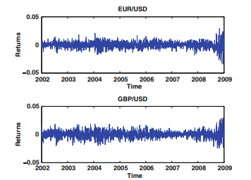
Exercise $3.4$ We consider a bivariate exchange rates example, two European currencies, EUR and GBP, with respect to the USD. The sample period is $01 / 01 / 2002$ to $01 / 01 / 2009$ with altogether $n=1,828$ observations. Figure $3.1$ shows the time series of returns on both exchange rates.
Compute the correlation of the two exchange rate time series and comment on the sign of the correlation.
Exercise 3.5 Compute the conditional moments $\mathrm{E}\left(X_{2} \mid x_{1}\right)$ and $\mathrm{E}\left(X_{1} \mid x_{2}\right)$ for the $p d f$ of
$$
f\left(x_{1}, x_{2}\right)=\left{\begin{array}{lc}
\frac{1}{2} x_{1}+\frac{3}{2} x_{2} & 0 \leq x_{1}, x_{2} \leq 1 \
0 & \text { otherwise }
\end{array}\right.
$$
Exercise $3.6$ Show that the function
$$
f_{Y}\left(y_{1}, y_{2}\right)= \begin{cases}\frac{1}{2} y_{1}-\frac{1}{4} y_{2} & 0 \leq y_{1} \leq 2,\left|y_{2}\right| \leq 1-\left|1-y_{1}\right| \ 0 & \text { otherwise }\end{cases}
$$
is a probability density function.
Exercise 3.7 Prove that $\mathrm{E} X_{2}=\mathrm{E}\left{\mathrm{E}\left(X_{2} \mid X_{1}\right)\right}$, where $\mathrm{E}\left(X_{2} \mid X_{1}\right)$ is the conditional expectation of $X_{2}$ given $X_{1}$.
Exercise 3.8 The conditional variance is defined as $\operatorname{Var}(Y \mid X)=\mathrm{E}[{Y-$ $\left.\mathrm{E}(Y \mid X)}^{2} \mid X\right]$. Show that $\operatorname{Var}(Y)=\mathrm{E}{\operatorname{Var}(Y \mid X)}+\operatorname{Var}{\mathrm{E}(Y \mid X)}$.
金融统计代写
统计代写|金融统计代写financial statistics代考|Random Vectors, Dependence, Correlation
随机向量(X1,…,Xn)从Rn可用于描述几个随机变量的相互依赖关系X1,…,Xn,例如几个标的股票。随机变量的联合分布X1,…,Xn与单变量情况一样,由概率唯一确定
磷(一种1≤X1≤b1,…,一种n≤Xn≤bn),−∞<一种一世≤b一世<∞,一世=1,…,n
如果随机向量(X1,…,Xn)有密度p(X1,…,Xn),概率可以通过以下积分计算:
磷(一种1≤X1≤b1,…,一种n≤Xn≤bn)=∫一种nbn…∫一种1b1p(X1,…,Xn)dX1…dXn
的单变量或边际分布Xj可以通过积分不感兴趣的变量从联合密度计算。
磷(一种j≤Xj≤bj)=∫−∞∞⋯∫一种jbj⋯∫−∞∞p(X1,…,Xn)dX1…dXn
两个随机变量独立的直观概念X1,X2通过要求正式化:
磷(一种1≤X1≤b1,一种2≤X2≤b2)=磷(一种1≤X1≤b1)⋅磷(一种2≤X2≤b2),
即两个事件的联合概率取决于随机向量(X1,X2)可以因式分解。考虑单变量分布就足够了X1和X2只。如果随机向量(X1,X2)有密度p(X1,X2), 然后X1和X2有密度p1(X)和p2(X)也是。在这种情况下,两个随机变量的独立性等价于可以分解的联合密度:
p(X1,X2)=p1(X1)p2(X2).
两个随机变量的相关性X1,X2可能非常复杂。如果X1,X2是联合正态分布的,它们的依赖结构可以很容易地通过它们的协方差来量化:
这(X1,X2)=和[(X1−和[X1])(X2−和[X2])],
统计代写|金融统计代写financial statistics代考|Conditional Probabilities and Expectations
随机变量的条件概率是取值之间一种和b条件是随机变量X取值之间X和X+ΔX, 定义为
磷(一种≤是≤b∣X≤X≤X+ΔX)=磷(一种≤是≤b,X≤X≤X+ΔX)磷(X≤X≤X+ΔX)
只要分母不为零。此类事件的条件概率一种≤是≤b反映了我们对哪些值比其他值更合理的看法,因为另一个随机变量X取了一定的值。如果是独立于X, 的概率是不受先验知识的影响X. 它拥有:
磷(一种≤是≤b∣X≤X≤X+ΔX)=磷(一种≤是≤b)
作为ΔX在等式中变为 0。(3.4),等式的左侧。(3.4) 启发式地收敛到磷(一种≤是≤b∣X=X). 在连续随机变量的情况下X有密度pX,等式的左侧。(3.4) 没有定义,因为磷(X=X)=0对全部X. 但是,可以给出条件分布的合理数学定义是给定X=X. 如果随机变量是和X有联合分布p(X,是),则条件分布有密度
p是∣X(是∣X)=p(X,是)pX(X) 为了 pX(X)≠0
和p是∣X(是∣X)=0除此以外。因此,它成立:
磷(一种≤是≤b∣X=X)=∫一种bp是∣X(是∣X)d是
关于条件分布的期望可以通过以下方式计算:
和(是∣X=X)=∫−∞∞是p是∣X(是∣X)d是= 定义 这(X)
统计代写|金融统计代写financial statistics代考|Recommended Literature
练习 3.1 检查随机变量X和磷(X=1)=1/2, 磷(X=−4)=1/3,磷(X=5)=1/6偏度为 0,但不是对称分布。
锻炼3.2证明如果这(X,是)=0这并不意味着X和是是独立的。
锻炼3.4我们考虑一个双变量汇率示例,两种欧洲货币,欧元和英镑,相对于美元。采样周期为01/01/2002到01/01/2009与共n=1,828观察。数字3.1显示两种汇率回报的时间序列。
计算两个汇率时间序列的相关性并评论相关性的符号。
练习 3.5 计算条件矩和(X2∣X1)和和(X1∣X2)为了pdF
$$ f\left (
x_{1}, x_{2}\right)=\left{12X1+32X20≤X1,X2≤1 0 除此以外 \对。
和X和rC一世s和$3.6$小号H这在吨H一种吨吨H和F在nC吨一世这n
f_{Y}\left(y_{1}, y_{2}\right)={12是1−14是20≤是1≤2,|是2|≤1−|1−是1| 0 除此以外
$$
是概率密度函数。
练习 3.7 证明\mathrm{E} X_{2}=\mathrm{E}\left{\mathrm{E}\left(X_{2} \mid X_{1}\right)\right}\mathrm{E} X_{2}=\mathrm{E}\left{\mathrm{E}\left(X_{2} \mid X_{1}\right)\right}, 在哪里和(X2∣X1)是条件期望X2给定X1.
练习 3.8 条件方差定义为\operatorname{Var}(Y \mid X)=\mathrm{E}[{Y-$ $\left.\mathrm{E}(Y \mid X)}^{2} \mid X\right]\operatorname{Var}(Y \mid X)=\mathrm{E}[{Y-$ $\left.\mathrm{E}(Y \mid X)}^{2} \mid X\right]. 显示曾是(是)=和曾是(是∣X)+曾是和(是∣X).

统计代写请认准statistics-lab™. statistics-lab™为您的留学生涯保驾护航。
金融工程代写
金融工程是使用数学技术来解决金融问题。金融工程使用计算机科学、统计学、经济学和应用数学领域的工具和知识来解决当前的金融问题,以及设计新的和创新的金融产品。
非参数统计代写
非参数统计指的是一种统计方法,其中不假设数据来自于由少数参数决定的规定模型;这种模型的例子包括正态分布模型和线性回归模型。
广义线性模型代考
广义线性模型(GLM)归属统计学领域,是一种应用灵活的线性回归模型。该模型允许因变量的偏差分布有除了正态分布之外的其它分布。
术语 广义线性模型(GLM)通常是指给定连续和/或分类预测因素的连续响应变量的常规线性回归模型。它包括多元线性回归,以及方差分析和方差分析(仅含固定效应)。
有限元方法代写
有限元方法(FEM)是一种流行的方法,用于数值解决工程和数学建模中出现的微分方程。典型的问题领域包括结构分析、传热、流体流动、质量运输和电磁势等传统领域。
有限元是一种通用的数值方法,用于解决两个或三个空间变量的偏微分方程(即一些边界值问题)。为了解决一个问题,有限元将一个大系统细分为更小、更简单的部分,称为有限元。这是通过在空间维度上的特定空间离散化来实现的,它是通过构建对象的网格来实现的:用于求解的数值域,它有有限数量的点。边界值问题的有限元方法表述最终导致一个代数方程组。该方法在域上对未知函数进行逼近。[1] 然后将模拟这些有限元的简单方程组合成一个更大的方程系统,以模拟整个问题。然后,有限元通过变化微积分使相关的误差函数最小化来逼近一个解决方案。
tatistics-lab作为专业的留学生服务机构,多年来已为美国、英国、加拿大、澳洲等留学热门地的学生提供专业的学术服务,包括但不限于Essay代写,Assignment代写,Dissertation代写,Report代写,小组作业代写,Proposal代写,Paper代写,Presentation代写,计算机作业代写,论文修改和润色,网课代做,exam代考等等。写作范围涵盖高中,本科,研究生等海外留学全阶段,辐射金融,经济学,会计学,审计学,管理学等全球99%专业科目。写作团队既有专业英语母语作者,也有海外名校硕博留学生,每位写作老师都拥有过硬的语言能力,专业的学科背景和学术写作经验。我们承诺100%原创,100%专业,100%准时,100%满意。
随机分析代写
随机微积分是数学的一个分支,对随机过程进行操作。它允许为随机过程的积分定义一个关于随机过程的一致的积分理论。这个领域是由日本数学家伊藤清在第二次世界大战期间创建并开始的。
时间序列分析代写
随机过程,是依赖于参数的一组随机变量的全体,参数通常是时间。 随机变量是随机现象的数量表现,其时间序列是一组按照时间发生先后顺序进行排列的数据点序列。通常一组时间序列的时间间隔为一恒定值(如1秒,5分钟,12小时,7天,1年),因此时间序列可以作为离散时间数据进行分析处理。研究时间序列数据的意义在于现实中,往往需要研究某个事物其随时间发展变化的规律。这就需要通过研究该事物过去发展的历史记录,以得到其自身发展的规律。
回归分析代写
多元回归分析渐进(Multiple Regression Analysis Asymptotics)属于计量经济学领域,主要是一种数学上的统计分析方法,可以分析复杂情况下各影响因素的数学关系,在自然科学、社会和经济学等多个领域内应用广泛。
MATLAB代写
MATLAB 是一种用于技术计算的高性能语言。它将计算、可视化和编程集成在一个易于使用的环境中,其中问题和解决方案以熟悉的数学符号表示。典型用途包括:数学和计算算法开发建模、仿真和原型制作数据分析、探索和可视化科学和工程图形应用程序开发,包括图形用户界面构建MATLAB 是一个交互式系统,其基本数据元素是一个不需要维度的数组。这使您可以解决许多技术计算问题,尤其是那些具有矩阵和向量公式的问题,而只需用 C 或 Fortran 等标量非交互式语言编写程序所需的时间的一小部分。MATLAB 名称代表矩阵实验室。MATLAB 最初的编写目的是提供对由 LINPACK 和 EISPACK 项目开发的矩阵软件的轻松访问,这两个项目共同代表了矩阵计算软件的最新技术。MATLAB 经过多年的发展,得到了许多用户的投入。在大学环境中,它是数学、工程和科学入门和高级课程的标准教学工具。在工业领域,MATLAB 是高效研究、开发和分析的首选工具。MATLAB 具有一系列称为工具箱的特定于应用程序的解决方案。对于大多数 MATLAB 用户来说非常重要,工具箱允许您学习和应用专业技术。工具箱是 MATLAB 函数(M 文件)的综合集合,可扩展 MATLAB 环境以解决特定类别的问题。可用工具箱的领域包括信号处理、控制系统、神经网络、模糊逻辑、小波、仿真等。