如果你也在 怎样代写金融统计Mathematics with Statistics for Finance G1GH这个学科遇到相关的难题,请随时右上角联系我们的24/7代写客服。
金融统计描述了应用数学和数学模型来解决金融问题。它有时被称为定量金融,金融工程,和计算金融。
statistics-lab™ 为您的留学生涯保驾护航 在代写金融统计Mathematics with Statistics for Finance G1GH方面已经树立了自己的口碑, 保证靠谱, 高质且原创的统计Statistics代写服务。我们的专家在代写金融统计Mathematics with Statistics for Finance G1GH方面经验极为丰富,各种代写金融统计Mathematics with Statistics for Finance G1GH相关的作业也就用不着说。
我们提供的金融统计Mathematics with Statistics for Finance G1GH及其相关学科的代写,服务范围广, 其中包括但不限于:
- Statistical Inference 统计推断
- Statistical Computing 统计计算
- Advanced Probability Theory 高等楖率论
- Advanced Mathematical Statistics 高等数理统计学
- (Generalized) Linear Models 广义线性模型
- Statistical Machine Learning 统计机器学习
- Longitudinal Data Analysis 纵向数据分析
- Foundations of Data Science 数据科学基础
统计代写|金融统计代写Mathematics with Statistics for Finance代考|LIMITED LIABILITY
Another useful feature of log returns relates to limited liability. For many financial assets, including equities and bonds, the most that you can lose is the amount that you’ve put into them. For example, if you purchase a share of $X Y Z$ Corporation for $\$ 100$, the most you can lose is that $\$ 100$. This is known as limited liability. Today, limited liability is such a common feature of financial instruments that it is easy to take it for granted, but this was not always the case. Indeed, the widespread adoption of limited liability in the nineteenth century made possible the large publicly traded companies that are so important to our modern economy, and the vast financial markets that accompany them.
That you can lose only your initial investment is equivalent to saying that the minimum possible return on your investment is $-100 \%$. At the other end of the spectrum, there is no upper limit to the amount you can make in an investment. The maximum possible return is, in theory, infinite. This range for simple returns, $-100 \%$ to infinity, translates to a range of negative infinity to positive infinity for log returns.
$$
\begin{aligned}
&R_{\min }=-100 \% \Rightarrow r_{\min }=-\infty \
&R_{\max }=+\infty \Rightarrow r_{\max }=+\infty
\end{aligned}
$$
As we will see in the following chapters, when it comes to mathematical and computer models in finance, it is often much easier to work with variables that are unbounded, that is variables that can range from negative infinity to positive infinity.
统计代写|金融统计代写Mathematics with Statistics for Finance代考|GRAPHING LOG RETURNS
Another useful feature of log returns is how they relate to log prices. By rearranging Equation $1.10$ and taking logs, it is easy to see that:
$$
r_{t}=p_{t}-p_{t-1}
$$
where $p_{t}$ is the log of $P_{t}$, the price at time $t$. To calculate log returns, rather than taking the log of one plus the simple return, we can simply calculate the logs of the prices and subtract.
Logarithms are also useful for charting time series that grow exponentially. Many computer applications allow you to chart data on a logarithmic scale. For an asset whose price grows exponentially, a logarithmic scale prevents the compression of data at low levels. Also, by rearranging Equation $1.13$, we can easily see that the change in the log price over time is equal to the log return:
$$
\Delta p_{t}=p_{t}-p_{t-1}=r_{t}
$$
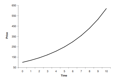
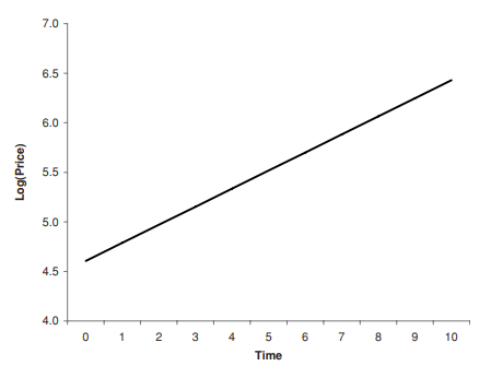
It follows that, for an asset whose return is constant, the change in the log price will also be constant over time. On a chart, this constant rate of change over time will translate into a constant slope. Figures $1.2$ and $1.3$ both show an asset whose price is increasing by $20 \%$ each year. The y-axis for the first chart shows the price; the $y$-axis for the second chart displays the log price.
For the chart in Figure $1.2$, it is hard to tell if the rate of return is increasing or decreasing over time. For the chart in Figure 1.3, the fact that
the line is straight is equivalent to saying that the line has a constant slope. From Equation $1.14$ we know that this constant slope is equivalent to a constant rate of return.
In the first chart, the $y$-axis could just have easily been the actual price (on a log scale), but having the log prices allows us to do something else. Using Equation 1.13, we can easily estimate the log return. Over 10 periods, the log price increases from approximately $4.6$ to $6.4$. Subtracting and dividing gives us $(6.4-4.6) / 10=18 \%$. So the log return is $18 \%$ per period, which-because log returns and simple returns are very close for small values-is very close to the actual simple return of $20 \%$.
统计代写|金融统计代写Mathematics with Statistics for Finance代考|CONTINUOUSLY COMPOUNDED RETURNS
Another topic related to the idea of log returns is continuously compounded returns. For many financial products, including bonds, mortgages, and credit cards, interest rates are often quoted on an annualized periodic or nominal basis. At each payment date, the amount to be paid is equal to this nominal rate, divided by the number of periods, multiplied by some notional amount.
For example, a bond with monthly coupon payments, a nominal rate of $6 \%$, and a notional value of $\$ 1,000$, would pay a coupon of $\$ 5$ each month: $(6 \% \times \$ 1,000) / 12=\$ 5$.
How do we compare two instruments with different payment frequencies? Are you better off paying $5 \%$ on an annual basis or $4.5 \%$ on a monthly basis? One solution is to turn the nominal rate into an annualized rate:
$$
R_{\text {Arnual }}=\left(1+\frac{R_{\text {Nominal }}}{n}\right)^{n}-1
$$
where $n$ is the number of periods per year for the instrument.
If we hold $R_{\text {Annual }}$ constant as $n$ increases, $R_{\text {Nominal gets smaller, but at }}$ a decreasing rate. Though the proof is omitted here, using L’Hôpital’s rule, we can prove that, at the limit, as $n$ approaches infinity, $R_{\text {Nominal converges }}$ to the log rate. As $n$ approaches infinity, it is as if the instrument is making infinitesimal payments on a continuous basis. Because of this, when used to define interest rates the log rate is often referred to as the continuously compounded rate, or simply the continuous rate. We can also compare two financial products with different payment periods by comparing their continuous rates.
金融统计代写
统计代写|金融统计代写Mathematics with Statistics for Finance代考|LIMITED LIABILITY
日志返回的另一个有用功能与有限责任有关。对于包括股票和债券在内的许多金融资产,您可能损失的最大金额是您投入其中的金额。例如,如果您购买了X是从公司为$100,你最多可以失去的是$100. 这被称为有限责任。今天,有限责任是金融工具的共同特征,人们很容易将其视为理所当然,但情况并非总是如此。事实上,有限责任在 19 世纪的广泛采用使得对我们现代经济如此重要的大型上市公司以及与之相伴的庞大金融市场成为可能。
你只能损失你的初始投资,就等于说你的投资的最低可能回报是−100%. 另一方面,您可以投资的金额没有上限。理论上,最大可能的回报是无限的。这个范围对于简单的回报,−100%到无穷大,转换为对数返回的负无穷大到正无穷大的范围。
R分钟=−100%⇒r分钟=−∞ R最大限度=+∞⇒r最大限度=+∞
正如我们将在接下来的章节中看到的,当涉及到金融中的数学和计算机模型时,使用无界变量通常要容易得多,即范围从负无穷到正无穷的变量。
统计代写|金融统计代写Mathematics with Statistics for Finance代考|GRAPHING LOG RETURNS
原木收益的另一个有用特征是它们与原木价格的关系。通过重新排列方程1.10并记录日志,很容易看出:
r吨=p吨−p吨−1
在哪里p吨是日志磷吨,当时的价格吨. 要计算对数收益,我们可以简单地计算价格的对数并减去,而不是取一加简单收益的对数。
对数也可用于绘制呈指数增长的时间序列。许多计算机应用程序允许您以对数刻度绘制数据。对于价格呈指数增长的资产,对数尺度可以防止数据在低水平上的压缩。此外,通过重新排列方程1.13,我们可以很容易地看出,原木价格随时间的变化等于原木收益:
Δp吨=p吨−p吨−1=r吨
由此可见,对于收益不变的资产,对数价格的变化也将随着时间的推移而保持不变。在图表上,这种随时间变化的恒定速率将转化为恒定斜率。数据1.2和1.3两者都显示价格上涨的资产20%每年。第一个图表的 y 轴显示价格;这是第二个图表的 – 轴显示对数价格。
对于图中的图表1.2,很难判断回报率是随时间增加还是减少。对于图 1.3 中的图表,事实是
这条线是直的,相当于说这条线有一个恒定的斜率。从方程1.14我们知道,这个恒定的斜率相当于一个恒定的回报率。
在第一张图表中,是-axis 可以很容易地成为实际价格(在对数刻度上),但是拥有对数价格可以让我们做其他事情。使用公式 1.13,我们可以轻松估计对数回报。在 10 个时期内,原木价格从大约4.6到6.4. 减法和除法给了我们(6.4−4.6)/10=18%. 所以日志返回是18%每个周期,因为日志回报和简单回报对于小值非常接近 – 非常接近实际的简单回报20%.
统计代写|金融统计代写Mathematics with Statistics for Finance代考|CONTINUOUSLY COMPOUNDED RETURNS
与对数回报概念相关的另一个主题是连续复合回报。对于许多金融产品,包括债券、抵押贷款和信用卡,利率通常按年化定期或名义报价。在每个付款日期,要支付的金额等于这个名义利率,除以期数,再乘以一些名义金额。
例如,按月支付息票的债券,名义利率为6%, 和一个名义价值$1,000, 会支付一张优惠券$5每一个月:(6%×$1,000)/12=$5.
我们如何比较两种支付频率不同的工具?你最好付钱吗5%每年一次或4.5%在每个月的基础上?一种解决方案是将名义利率转换为年化利率:
R年报 =(1+R标称 n)n−1
在哪里n是该工具每年的周期数。
如果我们持有R年度的 常数为n增加,R标称变小,但在 一个递减率。虽然这里省略了证明,但使用 L’Hôpital 规则,我们可以证明,在极限处,为n接近无穷大,R名义收敛 到对数率。作为n接近无穷大时,就好像该工具在连续进行无限小的支付。因此,当用于定义利率时,对数利率通常被称为连续复合利率,或简称为连续利率。我们还可以通过比较它们的连续费率来比较两种不同支付期限的金融产品。

统计代写请认准statistics-lab™. statistics-lab™为您的留学生涯保驾护航。统计代写|python代写代考
随机过程代考
在概率论概念中,随机过程是随机变量的集合。 若一随机系统的样本点是随机函数,则称此函数为样本函数,这一随机系统全部样本函数的集合是一个随机过程。 实际应用中,样本函数的一般定义在时间域或者空间域。 随机过程的实例如股票和汇率的波动、语音信号、视频信号、体温的变化,随机运动如布朗运动、随机徘徊等等。
贝叶斯方法代考
贝叶斯统计概念及数据分析表示使用概率陈述回答有关未知参数的研究问题以及统计范式。后验分布包括关于参数的先验分布,和基于观测数据提供关于参数的信息似然模型。根据选择的先验分布和似然模型,后验分布可以解析或近似,例如,马尔科夫链蒙特卡罗 (MCMC) 方法之一。贝叶斯统计概念及数据分析使用后验分布来形成模型参数的各种摘要,包括点估计,如后验平均值、中位数、百分位数和称为可信区间的区间估计。此外,所有关于模型参数的统计检验都可以表示为基于估计后验分布的概率报表。
广义线性模型代考
广义线性模型(GLM)归属统计学领域,是一种应用灵活的线性回归模型。该模型允许因变量的偏差分布有除了正态分布之外的其它分布。
statistics-lab作为专业的留学生服务机构,多年来已为美国、英国、加拿大、澳洲等留学热门地的学生提供专业的学术服务,包括但不限于Essay代写,Assignment代写,Dissertation代写,Report代写,小组作业代写,Proposal代写,Paper代写,Presentation代写,计算机作业代写,论文修改和润色,网课代做,exam代考等等。写作范围涵盖高中,本科,研究生等海外留学全阶段,辐射金融,经济学,会计学,审计学,管理学等全球99%专业科目。写作团队既有专业英语母语作者,也有海外名校硕博留学生,每位写作老师都拥有过硬的语言能力,专业的学科背景和学术写作经验。我们承诺100%原创,100%专业,100%准时,100%满意。
机器学习代写
随着AI的大潮到来,Machine Learning逐渐成为一个新的学习热点。同时与传统CS相比,Machine Learning在其他领域也有着广泛的应用,因此这门学科成为不仅折磨CS专业同学的“小恶魔”,也是折磨生物、化学、统计等其他学科留学生的“大魔王”。学习Machine learning的一大绊脚石在于使用语言众多,跨学科范围广,所以学习起来尤其困难。但是不管你在学习Machine Learning时遇到任何难题,StudyGate专业导师团队都能为你轻松解决。
多元统计分析代考
基础数据: $N$ 个样本, $P$ 个变量数的单样本,组成的横列的数据表
变量定性: 分类和顺序;变量定量:数值
数学公式的角度分为: 因变量与自变量
时间序列分析代写
随机过程,是依赖于参数的一组随机变量的全体,参数通常是时间。 随机变量是随机现象的数量表现,其时间序列是一组按照时间发生先后顺序进行排列的数据点序列。通常一组时间序列的时间间隔为一恒定值(如1秒,5分钟,12小时,7天,1年),因此时间序列可以作为离散时间数据进行分析处理。研究时间序列数据的意义在于现实中,往往需要研究某个事物其随时间发展变化的规律。这就需要通过研究该事物过去发展的历史记录,以得到其自身发展的规律。
回归分析代写
多元回归分析渐进(Multiple Regression Analysis Asymptotics)属于计量经济学领域,主要是一种数学上的统计分析方法,可以分析复杂情况下各影响因素的数学关系,在自然科学、社会和经济学等多个领域内应用广泛。
MATLAB代写
MATLAB 是一种用于技术计算的高性能语言。它将计算、可视化和编程集成在一个易于使用的环境中,其中问题和解决方案以熟悉的数学符号表示。典型用途包括:数学和计算算法开发建模、仿真和原型制作数据分析、探索和可视化科学和工程图形应用程序开发,包括图形用户界面构建MATLAB 是一个交互式系统,其基本数据元素是一个不需要维度的数组。这使您可以解决许多技术计算问题,尤其是那些具有矩阵和向量公式的问题,而只需用 C 或 Fortran 等标量非交互式语言编写程序所需的时间的一小部分。MATLAB 名称代表矩阵实验室。MATLAB 最初的编写目的是提供对由 LINPACK 和 EISPACK 项目开发的矩阵软件的轻松访问,这两个项目共同代表了矩阵计算软件的最新技术。MATLAB 经过多年的发展,得到了许多用户的投入。在大学环境中,它是数学、工程和科学入门和高级课程的标准教学工具。在工业领域,MATLAB 是高效研究、开发和分析的首选工具。MATLAB 具有一系列称为工具箱的特定于应用程序的解决方案。对于大多数 MATLAB 用户来说非常重要,工具箱允许您学习和应用专业技术。工具箱是 MATLAB 函数(M 文件)的综合集合,可扩展 MATLAB 环境以解决特定类别的问题。可用工具箱的领域包括信号处理、控制系统、神经网络、模糊逻辑、小波、仿真等。