如果你也在 怎样代写随机过程stochastic process这个学科遇到相关的难题,请随时右上角联系我们的24/7代写客服。
随机过程被定义为随机变量X={Xt:t∈T}的集合,定义在一个共同的概率空间上,在一个共同的集合S(状态空间)中取值,并以一个集合T为索引,通常是N或[0,∞],并被认为是时间(分别为离散或连续)。
statistics-lab™ 为您的留学生涯保驾护航 在代写随机过程stochastic process方面已经树立了自己的口碑, 保证靠谱, 高质且原创的统计Statistics代写服务。我们的专家在代写随机过程stochastic process代写方面经验极为丰富,各种代写随机过程stochastic process相关的作业也就用不着说。
我们提供的随机过程stochastic process及其相关学科的代写,服务范围广, 其中包括但不限于:
- Statistical Inference 统计推断
- Statistical Computing 统计计算
- Advanced Probability Theory 高等概率论
- Advanced Mathematical Statistics 高等数理统计学
- (Generalized) Linear Models 广义线性模型
- Statistical Machine Learning 统计机器学习
- Longitudinal Data Analysis 纵向数据分析
- Foundations of Data Science 数据科学基础
统计代写|随机过程代写stochastic process代考|The R script below simulates
EXERCISE 2.4. (a) The R script below simulates the trajectories and terminates them if the barrier is hit. Otherwise, trajectories continue for 1,000 steps. The total number of trajectories that hit the barrier is counted. We also record the number of steps (for part (b)) and the $y$-coordinate (for part (c)).
setting counter to zero
nhits<- 0
specifying seed
set.seed (50118)
defining walk as matrix
walk<- matrix (NA, nrow=1001, ncol=2)
nsteps<-c()
ycoord<- c()
defining random steps
Istep<- matrix $(c(1,0,-1,0,0,1,0,-1)$, nrow=4, ncol=2, byrow=TRUE)
simulating trajectories
for (j in 1:10000)
1
walk $[1,]<-c(0,0$, #setting initial value to the origin
for (i in 2:1001)
\&
walk $[i,]<-$, walk $[i-1,]+$, rstep $[\operatorname{sample}(1: 4, \operatorname{size}=1),$,
if $($ walk $[i, 1]==30) \quad$ {
nhits=nhits+1
break ?
1
nsteps [j]<- i
ycoord $[j]<-$ ifelse $(i==1001,99999$, walk $[i, 2])$
1
print (nhits)
1764
So, of the 10,000 trajectories, 1,764 hit the vertical barrier. Thus, the estimated probability to hit the barrier is $0.1764$.
(b) The average number of steps it takes a trajectory to hit the barrier, provided it did hit the barrier within the 1,000 steps, is estimated as
mean (nsteps [nsteps ! =1001])
$623.2053$
It took on average $623.2$ steps to hit the barrier for the $17.64 \%$ of the trajectories that terminated at the barrier.
(a) Estimate the expected value of the $y$-coordinate at the time when the random walk hits the barriet What should this value be from the theoretical point of view? Hint: deduce from a symmetry argument.
mean $($ ycoord $[$ ycoord $!=99999]))$
$0.1066364$
The estimated average $y$-coordinate for $17.64 \%$ of the trajectories that hit the barrier was $0.1066$. From the theoretical viewpoint, using the symmetry of the random walk, we can argue that the $y$ coordinate should be equal to 0 .
统计代写|随机过程代写stochastic process代考|By running the following script
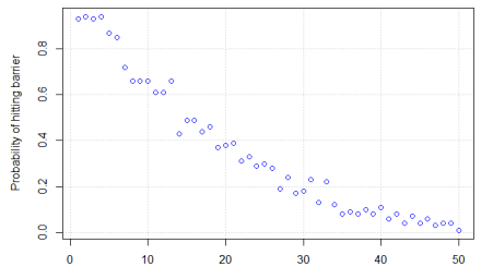
EXERCISE 2.5. By running the following script, we simulate trajectories and calculate the number of those that hit the barrier. The plot is given below.
Nhits<- c()
specifying seed
set.seed $(96770)$
defining walk as matrix
walk<- matrix (NA, nrow=1001, ncol=2)
defining random steps
rstep<- matrix $(c(1,0,-1,0,0,1,0,-1)$, nrow=4, ncol=2, byrow=TRUE $)$
varying the barrier value
for (barrier in $1: 50$ ) \&
nhits<- 0
Hyimulating trajectordes
for (j in 1:100)
1
walk $[1,]<-c(0,0$, #setting initial value to the origin
for (i in 2:1001)
{
walk $[1,]<-\operatorname{walk}[i-1,]+\operatorname{rstep}[\operatorname{sample}(1: 4, \operatorname{size}=1),$,
if (walk[i,1]==barrier) |
nhits=nhits+1
break ?
)
1
Nhits [barrier] =nhits
1
print (Nhits)
$$
\begin{array}{rrrrrrrrrrrrr}
{[1]} & 93 & 94 & 93 & 94 & 87 & 85 & 72 & 66 & 66 & 66 & 61 & 61 \
{[13]} & 66 & 43 & 49 & 49 & 44 & 46 & 37 & 38 & 39 & 31 & 33 & 29 \
{[25]} & 30 & 28 & 19 & 24 & 17 & 18 & 23 & 13 & 22 & 12 & 8 & 9 \
{[37]} & 8 & 10 & 8 & 11 & 6 & 8 & 4 & 7 & 4 & 6 & 3 & 4 \
{[49]} & 4 & 1 & & & & & & & & & &
\end{array}
$$
plot $(1: 50$, Nhits/100, col=”blue”, xlab=”Position of barrier”, ylab=”Probability of hitting barrier”, panel.first=grid())
统计代写|随机过程代写stochastic process代考|Conditioning on the outcome
EXERCISE 2.7. (a) Conditioning on the outcome of the first step, we see that the probability $\boldsymbol{P}{i}$ solves the recurrence relation $\boldsymbol{P}{i}=p \boldsymbol{P}{i+1}+q \boldsymbol{P}{i-1}$ with the border constraints $\boldsymbol{P}{A}=0$ and $\boldsymbol{P}{B}=1$. Assuming first that $\frac{q}{p} \neq 1$, we look for the solution in the form $\boldsymbol{P}{i}=c\left(\frac{q}{p}\right)^{i}+d$ where $c$ and $d$ are some constants that can be found from the boundary conditions: $\boldsymbol{P}{A}=0=c\left(\frac{q}{p}\right)^{A}+d$ and $\boldsymbol{P}{B}=1=$ $c\left(\frac{q}{p}\right)^{B}+d$. From here, $c=-\frac{1}{\left(\frac{q}{p}\right)^{\Lambda}-\left(\frac{q}{p}\right)^{B}}$ and $d=\frac{\left(\frac{q}{p}\right)^{A}}{\left(\frac{q}{p}\right)^{A}-\left(\frac{q}{p}\right)^{B}}$, and thus, $P{i}=\frac{\left(\frac{q}{p}\right)^{A}-\left(\frac{q}{p}\right)^{i}}{\left(\frac{q}{p}\right)^{A}-\left(\frac{q}{p}\right)^{B}}$.
Now assume $\frac{q}{p}=1$. We look for the solution of the recurrence relation in the form $\boldsymbol{P}{\ell}=c i+d$. Again, from the boundary conditions, $\boldsymbol{P}{A}=0=c A+d$ and $\boldsymbol{P}{B}=1=c B+d$. Hence, $c=\frac{1}{B-A}$ and $d=-\frac{A}{B-A}$, leading to $\boldsymbol{P}{i}=\frac{i-A}{B-A}$.
(b) By conditioning on the first step, we see right away that the expectation satisfies the recurrence relation $\boldsymbol{E}{i}=p \boldsymbol{E}{i+1}+q \boldsymbol{E}{i-1}+1$ with the boundary conditions $E{A}=E_{B}=0$. Because of the additive constant term, this equation is referred to as a non-homogeneous relation and the general solution is sought in the form $\boldsymbol{E}{i}=c\left(\frac{q}{p}\right)^{i}+d+\frac{i}{q-p}$, if $\frac{q}{p} \neq 1$, and $\boldsymbol{E}{i}=c i+d-i^{2}$, if $\frac{q}{p}=1$. The constants $c$ and $d$ are found from the boundary conditions. In the former case, they satisfy $\boldsymbol{E}{A}=0=c\left(\frac{q}{p}\right)^{A}+d+\frac{A}{q-p}$ and $\boldsymbol{E}{B}=0=c\left(\frac{q}{p}\right)^{B}+d+\frac{B}{q-p}$. Whence,
$$
c=\frac{B-A}{q-p} \cdot \frac{1}{\left(\frac{q}{p}\right)^{A}-\left(\frac{q}{p}\right)^{B}},
$$
and
$$
d=-\frac{B-A}{q-p} \cdot \frac{\left(\frac{q}{p}\right)^{B}}{\left(\frac{q}{p}\right)^{A}-\left(\frac{q}{p}\right)^{B}}-\frac{B}{q-p}
$$
resulting in
$$
\boldsymbol{E}{i}=\frac{B-A}{q-p} \cdot \frac{\left(\frac{q}{p}\right)^{i}-\left(\frac{q}{p}\right)^{B}}{\left(\frac{q}{p}\right)^{A}-\left(\frac{q}{p}\right)^{B}}-\frac{B-i}{q-p} $$ In the latter case, $c$ and $d$ solve $E{A}=0=c A+d-A^{2}$ and $E_{B}=0=c B+d-B^{2}$. From here, $c=A+B$ and $d=-A B$. Thus, $\boldsymbol{E}{i}=(A+B) i-A B-i^{2}=(B-i)(i-A)$. (c) We use the formulas derived above with $p=0.47, q=0.53, A=10, i=40$, and $B=80$. We obtain $$ \boldsymbol{P}{40}=\frac{\left(\frac{0.53}{0.47}\right)^{10}-\left(\frac{0.53}{0.47}\right)^{40}}{\left(\frac{0.53}{0.47}\right)^{10}-\left(\frac{0.53}{0.47}\right)^{80}}=0.007962
$$
and
$$
\boldsymbol{E}_{40}=\frac{80-10}{0.53-0.47} \cdot \frac{\left(\frac{0.53}{0.47}\right)^{40}-\left(\frac{0.53}{0.47}\right)^{80}}{\left(\frac{0.53}{0.47}\right)^{10}-\left(\frac{0.53}{0.47}\right)^{80}}-\frac{80-40}{0.53-0.47}=490.7115
$$
The probability of doubling the fortune in this rigged game is very small (about $0.008$ ), and the gambler will play, on average, about 491 games before he walks out of the casino.
随机过程代写
统计代写|随机过程代写stochastic process代考|The R script below simulates
练习 2.4。(a) 下面的 R 脚本模拟轨迹并在遇到障碍时终止它们。否则,轨迹将持续 1,000 步。计算撞击障碍物的轨迹总数。我们还记录了步数(对于(b)部分)和是-坐标(对于(c)部分)。
将计数器设置为零
n命中<- 0
指定种子
set.seed (50118)
将walk定义为矩阵
walk<- 矩阵 (NA, nrow=1001, ncol=2)
nsteps<-c()
ycoord<- c()
定义随机步骤
Istep<- 矩阵(C(1,0,−1,0,0,1,0,−1), nrow=4, ncol=2, byrow=TRUE)
模拟轨迹
为 (j in 1:10000)
1
次步行[1,]<−C(0,0, #setting initial value to the origin
for (i in 2:1001)
\&
walk[一世,]<−, 走[一世−1,]+, r 步[样本(1:4,尺寸=1),,
如果(走[一世,1]==30){
nhits=nhits+1
中断 ?
1
nsteps [j]<- i
ycoord[j]<−如果别的(一世==1001,99999, 走[一世,2])
1
print (nhits)
1764
因此,在 10,000 条轨迹中,有 1,764 条击中了垂直屏障。因此,估计撞到障碍物的概率是0.1764.
(b) 轨迹撞到障碍物的平均步数,假设它确实在 1,000 步内撞到障碍物,估计为
平均值 (nsteps [nsteps ! =1001])
623.2053
平均花费了623.2击中障碍的步骤17.64%在障碍物处终止的轨迹。
(a) 估计预期值是- 随机游走击中 barriet 时的坐标 从理论的角度来看,这个值应该是多少?提示:从对称论证中推导出来。
意思是(ycoord[ycoord!=99999]))
0.1066364
估计平均值是- 坐标17.64%撞击障碍物的轨迹是0.1066. 从理论的角度来看,利用随机游走的对称性,我们可以认为是坐标应等于 0 。
统计代写|随机过程代写stochastic process代考|By running the following script
练习 2.5。通过运行以下脚本,我们可以模拟轨迹并计算撞击障碍物的数量。情节如下。
Nhits<-c()
指定种子
设置种子(96770)
将walk定义为矩阵
walk<- 矩阵(NA,nrow=1001,ncol=2)
定义随机步骤
rstep<- 矩阵(C(1,0,−1,0,0,1,0,−1), nrow=4, ncol=2, byrow=TRUE)
改变障碍值
对于(障碍在1:50) \&
nhits<- 0
Hyimulating 轨迹
为 (j in 1:100)
1
walk[1,]<−C(0,0, #将初始值设置为原点
for (i in 2:1001)
{
walk[1,]<−走[一世−1,]+rstep[样本(1:4,尺寸=1),,
if (walk[i,1]==barrier) |
nhits=nhits+1
中断?
)
1
Nhits [障碍] =nhits
1
打印(Nhits)
[1]939493948785726666666161 [13]664349494446373839313329 [25]3028192417182313221289 [37]81081168474634 [49]41
阴谋(1:50, Nhits/100, col=”blue”, xlab=”屏障位置”, ylab=”击中屏障的概率”, panel.first=grid())
统计代写|随机过程代写stochastic process代考|Conditioning on the outcome
练习 2.7。(a) 以第一步的结果为条件,我们看到概率磷一世解决递归关系磷一世=p磷一世+1+q磷一世−1有边界约束磷一种=0和磷乙=1. 首先假设qp≠1,我们在表格中寻找解决方案磷一世=C(qp)一世+d在哪里C和d是一些可以从边界条件中找到的常数:磷一种=0=C(qp)一种+d和磷乙=1= C(qp)乙+d. 从这里,C=−1(qp)Λ−(qp)乙和d=(qp)一种(qp)一种−(qp)乙, 因此,磷一世=(qp)一种−(qp)一世(qp)一种−(qp)乙.
现在假设qp=1. 我们以形式寻找递推关系的解磷ℓ=C一世+d. 再次,从边界条件,磷一种=0=C一种+d和磷乙=1=C乙+d. 因此,C=1乙−一种和d=−一种乙−一种, 导致磷一世=一世−一种乙−一种.
(b) 通过以第一步为条件,我们立即看到期望满足递归关系和一世=p和一世+1+q和一世−1+1有边界条件和一种=和乙=0. 由于附加常数项,该方程被称为非齐次关系,并以形式寻求通解和一世=C(qp)一世+d+一世q−p, 如果qp≠1, 和和一世=C一世+d−一世2, 如果qp=1. 常数C和d由边界条件求得。在前一种情况下,它们满足和一种=0=C(qp)一种+d+一种q−p和和乙=0=C(qp)乙+d+乙q−p. 何处,
C=乙−一种q−p⋅1(qp)一种−(qp)乙,
和
d=−乙−一种q−p⋅(qp)乙(qp)一种−(qp)乙−乙q−p
导致和一世=乙−一种q−p⋅(qp)一世−(qp)乙(qp)一种−(qp)乙−乙−一世q−p在后一种情况下,C和d解决和一种=0=C一种+d−一种2和和乙=0=C乙+d−乙2. 从这里,C=一种+乙和d=−一种乙. 因此,和一世=(一种+乙)一世−一种乙−一世2=(乙−一世)(一世−一种). (c) 我们使用上面推导的公式p=0.47,q=0.53,一种=10,一世=40, 和乙=80. 我们获得磷40=(0.530.47)10−(0.530.47)40(0.530.47)10−(0.530.47)80=0.007962
和
和40=80−100.53−0.47⋅(0.530.47)40−(0.530.47)80(0.530.47)10−(0.530.47)80−80−400.53−0.47=490.7115
在这个被操纵的游戏中,财富翻倍的概率非常小(大约0.008),赌徒在走出赌场之前平均会玩大约 491 场游戏。

统计代写请认准statistics-lab™. statistics-lab™为您的留学生涯保驾护航。
金融工程代写
金融工程是使用数学技术来解决金融问题。金融工程使用计算机科学、统计学、经济学和应用数学领域的工具和知识来解决当前的金融问题,以及设计新的和创新的金融产品。
非参数统计代写
非参数统计指的是一种统计方法,其中不假设数据来自于由少数参数决定的规定模型;这种模型的例子包括正态分布模型和线性回归模型。
广义线性模型代考
广义线性模型(GLM)归属统计学领域,是一种应用灵活的线性回归模型。该模型允许因变量的偏差分布有除了正态分布之外的其它分布。
术语 广义线性模型(GLM)通常是指给定连续和/或分类预测因素的连续响应变量的常规线性回归模型。它包括多元线性回归,以及方差分析和方差分析(仅含固定效应)。
有限元方法代写
有限元方法(FEM)是一种流行的方法,用于数值解决工程和数学建模中出现的微分方程。典型的问题领域包括结构分析、传热、流体流动、质量运输和电磁势等传统领域。
有限元是一种通用的数值方法,用于解决两个或三个空间变量的偏微分方程(即一些边界值问题)。为了解决一个问题,有限元将一个大系统细分为更小、更简单的部分,称为有限元。这是通过在空间维度上的特定空间离散化来实现的,它是通过构建对象的网格来实现的:用于求解的数值域,它有有限数量的点。边界值问题的有限元方法表述最终导致一个代数方程组。该方法在域上对未知函数进行逼近。[1] 然后将模拟这些有限元的简单方程组合成一个更大的方程系统,以模拟整个问题。然后,有限元通过变化微积分使相关的误差函数最小化来逼近一个解决方案。
tatistics-lab作为专业的留学生服务机构,多年来已为美国、英国、加拿大、澳洲等留学热门地的学生提供专业的学术服务,包括但不限于Essay代写,Assignment代写,Dissertation代写,Report代写,小组作业代写,Proposal代写,Paper代写,Presentation代写,计算机作业代写,论文修改和润色,网课代做,exam代考等等。写作范围涵盖高中,本科,研究生等海外留学全阶段,辐射金融,经济学,会计学,审计学,管理学等全球99%专业科目。写作团队既有专业英语母语作者,也有海外名校硕博留学生,每位写作老师都拥有过硬的语言能力,专业的学科背景和学术写作经验。我们承诺100%原创,100%专业,100%准时,100%满意。
随机分析代写
随机微积分是数学的一个分支,对随机过程进行操作。它允许为随机过程的积分定义一个关于随机过程的一致的积分理论。这个领域是由日本数学家伊藤清在第二次世界大战期间创建并开始的。
时间序列分析代写
随机过程,是依赖于参数的一组随机变量的全体,参数通常是时间。 随机变量是随机现象的数量表现,其时间序列是一组按照时间发生先后顺序进行排列的数据点序列。通常一组时间序列的时间间隔为一恒定值(如1秒,5分钟,12小时,7天,1年),因此时间序列可以作为离散时间数据进行分析处理。研究时间序列数据的意义在于现实中,往往需要研究某个事物其随时间发展变化的规律。这就需要通过研究该事物过去发展的历史记录,以得到其自身发展的规律。
回归分析代写
多元回归分析渐进(Multiple Regression Analysis Asymptotics)属于计量经济学领域,主要是一种数学上的统计分析方法,可以分析复杂情况下各影响因素的数学关系,在自然科学、社会和经济学等多个领域内应用广泛。
MATLAB代写
MATLAB 是一种用于技术计算的高性能语言。它将计算、可视化和编程集成在一个易于使用的环境中,其中问题和解决方案以熟悉的数学符号表示。典型用途包括:数学和计算算法开发建模、仿真和原型制作数据分析、探索和可视化科学和工程图形应用程序开发,包括图形用户界面构建MATLAB 是一个交互式系统,其基本数据元素是一个不需要维度的数组。这使您可以解决许多技术计算问题,尤其是那些具有矩阵和向量公式的问题,而只需用 C 或 Fortran 等标量非交互式语言编写程序所需的时间的一小部分。MATLAB 名称代表矩阵实验室。MATLAB 最初的编写目的是提供对由 LINPACK 和 EISPACK 项目开发的矩阵软件的轻松访问,这两个项目共同代表了矩阵计算软件的最新技术。MATLAB 经过多年的发展,得到了许多用户的投入。在大学环境中,它是数学、工程和科学入门和高级课程的标准教学工具。在工业领域,MATLAB 是高效研究、开发和分析的首选工具。MATLAB 具有一系列称为工具箱的特定于应用程序的解决方案。对于大多数 MATLAB 用户来说非常重要,工具箱允许您学习和应用专业技术。工具箱是 MATLAB 函数(M 文件)的综合集合,可扩展 MATLAB 环境以解决特定类别的问题。可用工具箱的领域包括信号处理、控制系统、神经网络、模糊逻辑、小波、仿真等。