如果你也在 怎样代写风险建模Financial risk modeling这个学科遇到相关的难题,请随时右上角联系我们的24/7代写客服。
风险建模是确定有多少风险存在于一个特定的企业、投资或一系列的现金流中。
statistics-lab™ 为您的留学生涯保驾护航 在代写风险建模Financial risk modeling方面已经树立了自己的口碑, 保证靠谱, 高质且原创的统计Statistics代写服务。我们的专家在代写风险建模Financial risk modeling代写方面经验极为丰富,各种代写风险建模Financial risk modeling相关的作业也就用不着说。
我们提供的风险建模Financial risk modeling及其相关学科的代写,服务范围广, 其中包括但不限于:
- Statistical Inference 统计推断
- Statistical Computing 统计计算
- Advanced Probability Theory 高等楖率论
- Advanced Mathematical Statistics 高等数理统计学
- (Generalized) Linear Models 广义线性模型
- Statistical Machine Learning 统计机器学习
- Longitudinal Data Analysis 纵向数据分析
- Foundations of Data Science 数据科学基础

统计代写|风险建模代写Financial risk modeling代考|The timeline of a limit order history
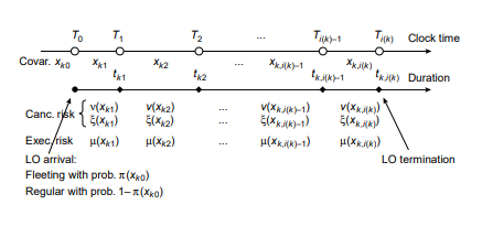
A stylized timeline of the limit order history is shown on the next page. The first row marks the clock time $T_{i}$ (measured in seconds since start of the trading day), the second row marks the time $t_{k i}$ since the moment $t_{k 0}$ of $k$ th limit order arrival, the third row marks $i(k)$ duration episodes $\Delta t_{k i}$ between consecutive changes of covariates $x_{k i}$ and the fourth row shows the values of time-varying covariates immediately before the beginning of each new episode of the limit order history. Row five shows the hazard rate $v\left(x_{k 0}\right)$ of cancellation for fleeting orders, row six shows the hazard rate $\xi\left(x_{k i}\right)$ of cancellation for regular (non-fleeting) limit orders and row seven shows the hazard rate $\mu\left(\boldsymbol{x}{k i}\right) R\left(\boldsymbol{x}{k i}\right)$ of order execution in each of the durations prior to the $k$ th limit order termination.
统计代写|风险建模代写Financial risk modeling代考|The likelihood function
To derive the expression for the likelihood function $L_{k}$ of $k$ th limit order, we start with the model where the risks of execution and cancellation are conditionally independent given the values of covariates. Then we show how the derived log-likelihood function can be maximized by standard methods of survival analysis, since the likelihood function $L_{k}$ can be decomposed into the product of two terms, $L_{c k}$ and $L_{e k}$, corresponding to the likelihood terms of cancellation and execution risks. The likelihood function of cancellation can be written as follows:
$$
\begin{aligned}
L_{c k}(\pi, v, \xi)=& \frac{e^{-\pi^{\prime} x_{k 0}}}{1+e^{-\pi^{\prime} x_{k 0}}} \exp \left[\sum_{i=1}^{i(k)}\left(\delta_{k i} \ln v\left(x_{k 0}\right)-v\left(x_{k 0}\right) \Delta t_{k i}\right)\right] \
&+\frac{1}{1+e^{-\pi^{\prime} x_{k 0}}} \exp \left[\sum_{i=1}^{i(k)}\left(\delta_{k i} \ln \xi\left(x_{k i}\right)-\xi\left(x_{k i}\right) \Delta t_{k i}\right)\right]
\end{aligned}
$$
where $\delta_{k i}$ is the indicator of the event that ith duration episode is terminated by cancellation. The likelihood function of execution is written similarly as:
$$
L_{e k}(\mu)=\exp \left[\sum_{i=1}^{i(k)}\left(d_{k i} \ln \mu\left(x_{k i}\right)-R\left(x_{k i}\right) \mu\left(x_{k i}\right) \Delta t_{k i}\right)\right]
$$
where $d_{k i}$ is the indicator of the event that ith duration episode is terminated by execution.
The log-likelihood function corresponding to the cancellation risk can be written in the additive form as follows:
$$
\begin{aligned}
\ln L_{c k}(\pi, v, \xi)=&-\left(\pi^{\prime} x_{k 0}+\ln \left(1+e^{-\pi^{\prime} x_{k 0}}\right)+\ln \left(1+Z_{c k}(\pi, v, \xi)\right)\right) \
&+\sum_{i=1}^{i(k)}\left(\delta_{k i} \ln v\left(x_{k 0}\right)-v\left(x_{k 0}\right) \Delta t_{k i}\right)
\end{aligned}
$$
where
$$
Z_{c k}(\pi, v, \xi)=\pi^{\prime} x_{k 0}+\sum_{i=1}^{i(k)}\left(\delta_{k i} y_{k i}-v\left(x_{k 0}\right)\left(1-e^{y_{k i}}\right)\right)
$$
and
$$
y_{k i}=\ln \xi\left(x_{k i}\right)-\ln v\left(x_{k 0}\right) .
$$
The log-likelihood function corresponding to execution risk is written similarly as follows:
$$
\ln L_{e k}(\mu)=\sum_{i=1}^{i(k)}\left(d_{k i} \ln \mu\left(x_{k i}\right)-R\left(x_{k i}\right) \mu\left(x_{k i}\right) \Delta t_{k i}\right)
$$
统计代写|风险建模代写Financial risk modeling代考|Estimation results
Panel A of Table $2.7$ shows the results for the model of intensity of limit order arrival at best quotes for ask orders for 13 randomly chosen stocks and Panel B shows the same for the mixture model for cancellation of limit orders arriving at best quotes. Estimates that have the same sign at least 90 percent of the days are boldfaced.
Panel $B$ shows that the probability of a fleeting order at best ask quotes depends:
- positively on bid-ask spread,
- positively on recent buyer-initiated trading volume (in the last 5 seconds),
- positively (but not as strongly) on recent (last 5 seconds) executions of hidden bid orders,
- negatively on LOB depth at and near the best quote on the same side,
- negatively (except for ISRG) on LOB depth at best quote on the opposite side,
- negatively for small relative spread stocks (AAPL, CMCSA) and positively for larger relative spread stocks (AKAM, GOOG, ISRG) on recent (in the last five seconds) seller-initiated trading volume.
The intensity of limit order arrival at best ask quotes (shown in Panel A)
- depends positively on bid-ask spread,
- depends positively on recent (in the last five seconds) buyer- and seller-initiated trading volume, although more strongly on sellerinitiated trading volume,
- depends negatively on LOB depth at and near the best quote on the opposite side,
- exhibits positive dependence on LOB depth near the same side best quote for AMGN and ISRG and negative dependence on LOB depth near the same side best quote for CMCSA.
风险建模代写
统计代写|风险建模代写Financial risk modeling代考|The timeline of a limit order history
限价单历史的程式化时间线显示在下一页。第一行标记时钟时间吨一世(以交易日开始后的秒数为单位),第二行标记时间吨ķ一世从那一刻起吨ķ0的ķ限价单到货,第三排标记一世(ķ)持续时间剧集Δ吨ķ一世在协变量的连续变化之间Xķ一世第四行显示限价单历史的每个新片段开始之前的时变协变量值。第五行显示危险率在(Xķ0)取消转瞬即逝的订单,第 6 行显示危险率X(Xķ一世)常规(非暂时性)限价单的取消,第 7 行显示危险率μ(Xķ一世)R(Xķ一世)在之前的每个持续时间的订单执行ķ限价单终止。
统计代写|风险建模代写Financial risk modeling代考|The likelihood function
导出似然函数的表达式大号ķ的ķ对于限价单,我们从模型开始,其中执行和取消的风险在给定协变量值的情况下是条件独立的。然后我们展示了如何通过标准的生存分析方法最大化导出的对数似然函数,因为似然函数大号ķ可以分解为两项的乘积,大号Cķ和大号和ķ,对应于取消和执行风险的可能性条款。抵消的似然函数可以写成如下:
大号Cķ(圆周率,在,X)=和−圆周率′Xķ01+和−圆周率′Xķ0经验[∑一世=1一世(ķ)(dķ一世ln在(Xķ0)−在(Xķ0)Δ吨ķ一世)] +11+和−圆周率′Xķ0经验[∑一世=1一世(ķ)(dķ一世lnX(Xķ一世)−X(Xķ一世)Δ吨ķ一世)]
在哪里dķ一世是第 i 个持续时间情节因取消而终止的事件的指示符。执行的似然函数类似地写成:
大号和ķ(μ)=经验[∑一世=1一世(ķ)(dķ一世lnμ(Xķ一世)−R(Xķ一世)μ(Xķ一世)Δ吨ķ一世)]
在哪里dķ一世是第 i 个持续时间的情节被执行终止的事件的指标。
取消风险对应的对数似然函数可以写成加法形式如下:
ln大号Cķ(圆周率,在,X)=−(圆周率′Xķ0+ln(1+和−圆周率′Xķ0)+ln(1+从Cķ(圆周率,在,X))) +∑一世=1一世(ķ)(dķ一世ln在(Xķ0)−在(Xķ0)Δ吨ķ一世)
在哪里
从Cķ(圆周率,在,X)=圆周率′Xķ0+∑一世=1一世(ķ)(dķ一世是ķ一世−在(Xķ0)(1−和是ķ一世))
和
是ķ一世=lnX(Xķ一世)−ln在(Xķ0).
执行风险对应的对数似然函数写法类似如下:
ln大号和ķ(μ)=∑一世=1一世(ķ)(dķ一世lnμ(Xķ一世)−R(Xķ一世)μ(Xķ一世)Δ吨ķ一世)
统计代写|风险建模代写Financial risk modeling代考|Estimation results
表 A 面板2.7显示了 13 只随机选择的股票的卖出订单的限价订单到达最佳报价强度模型的结果,面板 B 显示了取消到达最佳报价的限价订单的混合模型的相同结果。至少 90% 的天数具有相同符号的估计值以粗体显示。
控制板乙表明转瞬即逝的订单充其量要价的概率取决于:
- 积极的买卖差价,
- 对近期买家发起的交易量(在最后 5 秒内)持积极态度,
- 对最近(最后 5 秒)隐藏的投标订单执行积极(但不那么强烈),
- 在同一侧的最佳报价处和附近对 LOB 深度产生负面影响,
- 负面(ISRG 除外)对 LOB 深度的最佳报价在另一侧,
- 在最近(过去 5 秒内)卖方发起的交易量中,对相对价差较小的股票(AAPL、CMCSA)不利,对价差较大的股票(AKAM、GOOG、ISRG)有利。
限价单到达最佳卖价的强度(如面板 A 所示)
- 正依赖于买卖差价,
- 积极地取决于最近(在最后 5 秒内)买方和卖方发起的交易量,尽管更强烈地取决于卖方发起的交易量,
- 负面取决于对面最佳报价处和附近的 LOB 深度,
- 对 AMGN 和 ISRG 的同侧最佳报价附近的 LOB 深度表现出正相关性,对 CMCSA 的同侧最佳报价附近的 LOB 深度表现出负相关性。

统计代写请认准statistics-lab™. statistics-lab™为您的留学生涯保驾护航。
金融工程代写
金融工程是使用数学技术来解决金融问题。金融工程使用计算机科学、统计学、经济学和应用数学领域的工具和知识来解决当前的金融问题,以及设计新的和创新的金融产品。
非参数统计代写
非参数统计指的是一种统计方法,其中不假设数据来自于由少数参数决定的规定模型;这种模型的例子包括正态分布模型和线性回归模型。
广义线性模型代考
广义线性模型(GLM)归属统计学领域,是一种应用灵活的线性回归模型。该模型允许因变量的偏差分布有除了正态分布之外的其它分布。
术语 广义线性模型(GLM)通常是指给定连续和/或分类预测因素的连续响应变量的常规线性回归模型。它包括多元线性回归,以及方差分析和方差分析(仅含固定效应)。
有限元方法代写
有限元方法(FEM)是一种流行的方法,用于数值解决工程和数学建模中出现的微分方程。典型的问题领域包括结构分析、传热、流体流动、质量运输和电磁势等传统领域。
有限元是一种通用的数值方法,用于解决两个或三个空间变量的偏微分方程(即一些边界值问题)。为了解决一个问题,有限元将一个大系统细分为更小、更简单的部分,称为有限元。这是通过在空间维度上的特定空间离散化来实现的,它是通过构建对象的网格来实现的:用于求解的数值域,它有有限数量的点。边界值问题的有限元方法表述最终导致一个代数方程组。该方法在域上对未知函数进行逼近。[1] 然后将模拟这些有限元的简单方程组合成一个更大的方程系统,以模拟整个问题。然后,有限元通过变化微积分使相关的误差函数最小化来逼近一个解决方案。
tatistics-lab作为专业的留学生服务机构,多年来已为美国、英国、加拿大、澳洲等留学热门地的学生提供专业的学术服务,包括但不限于Essay代写,Assignment代写,Dissertation代写,Report代写,小组作业代写,Proposal代写,Paper代写,Presentation代写,计算机作业代写,论文修改和润色,网课代做,exam代考等等。写作范围涵盖高中,本科,研究生等海外留学全阶段,辐射金融,经济学,会计学,审计学,管理学等全球99%专业科目。写作团队既有专业英语母语作者,也有海外名校硕博留学生,每位写作老师都拥有过硬的语言能力,专业的学科背景和学术写作经验。我们承诺100%原创,100%专业,100%准时,100%满意。
随机分析代写
随机微积分是数学的一个分支,对随机过程进行操作。它允许为随机过程的积分定义一个关于随机过程的一致的积分理论。这个领域是由日本数学家伊藤清在第二次世界大战期间创建并开始的。
时间序列分析代写
随机过程,是依赖于参数的一组随机变量的全体,参数通常是时间。 随机变量是随机现象的数量表现,其时间序列是一组按照时间发生先后顺序进行排列的数据点序列。通常一组时间序列的时间间隔为一恒定值(如1秒,5分钟,12小时,7天,1年),因此时间序列可以作为离散时间数据进行分析处理。研究时间序列数据的意义在于现实中,往往需要研究某个事物其随时间发展变化的规律。这就需要通过研究该事物过去发展的历史记录,以得到其自身发展的规律。
回归分析代写
多元回归分析渐进(Multiple Regression Analysis Asymptotics)属于计量经济学领域,主要是一种数学上的统计分析方法,可以分析复杂情况下各影响因素的数学关系,在自然科学、社会和经济学等多个领域内应用广泛。
MATLAB代写
MATLAB 是一种用于技术计算的高性能语言。它将计算、可视化和编程集成在一个易于使用的环境中,其中问题和解决方案以熟悉的数学符号表示。典型用途包括:数学和计算算法开发建模、仿真和原型制作数据分析、探索和可视化科学和工程图形应用程序开发,包括图形用户界面构建MATLAB 是一个交互式系统,其基本数据元素是一个不需要维度的数组。这使您可以解决许多技术计算问题,尤其是那些具有矩阵和向量公式的问题,而只需用 C 或 Fortran 等标量非交互式语言编写程序所需的时间的一小部分。MATLAB 名称代表矩阵实验室。MATLAB 最初的编写目的是提供对由 LINPACK 和 EISPACK 项目开发的矩阵软件的轻松访问,这两个项目共同代表了矩阵计算软件的最新技术。MATLAB 经过多年的发展,得到了许多用户的投入。在大学环境中,它是数学、工程和科学入门和高级课程的标准教学工具。在工业领域,MATLAB 是高效研究、开发和分析的首选工具。MATLAB 具有一系列称为工具箱的特定于应用程序的解决方案。对于大多数 MATLAB 用户来说非常重要,工具箱允许您学习和应用专业技术。工具箱是 MATLAB 函数(M 文件)的综合集合,可扩展 MATLAB 环境以解决特定类别的问题。可用工具箱的领域包括信号处理、控制系统、神经网络、模糊逻辑、小波、仿真等。