如果你也在 怎样代写Generalized linear model这个学科遇到相关的难题,请随时右上角联系我们的24/7代写客服。
广义线性模型(GLiM,或GLM)是John Nelder和Robert Wedderburn在1972年提出的一种高级统计建模技术。它是一个包括许多其他模型的总称,它允许响应变量y具有正态分布以外的误差分布。
statistics-lab™ 为您的留学生涯保驾护航 在代写Generalized linear model方面已经树立了自己的口碑, 保证靠谱, 高质且原创的统计Statistics代写服务。我们的专家在代写Generalized linear model代写方面经验极为丰富,各种代写Generalized linear model相关的作业也就用不着说。
我们提供的Generalized linear model及其相关学科的代写,服务范围广, 其中包括但不限于:
- Statistical Inference 统计推断
- Statistical Computing 统计计算
- Advanced Probability Theory 高等概率论
- Advanced Mathematical Statistics 高等数理统计学
- (Generalized) Linear Models 广义线性模型
- Statistical Machine Learning 统计机器学习
- Longitudinal Data Analysis 纵向数据分析
- Foundations of Data Science 数据科学基础
统计代写|Generalized linear model代考广义线性模型代写|Linear Transformations
To perform a linear transformation, you need to take a dataset and either add, subtract, multiply, or divide every score by the same constant. (You may remember from Chapter 1 that a constant is a score that is the same for every member of a sample or population.) Performing a linear transformation is common in statistics. Linear transformations change the data, and that means they can have an impact on models derived from the data – including visual models and descriptive statistics.
Linear transformations allow us to convert data from one scale to a more preferable scale. For example, converting measurements recorded in inches into centimeters requires a linear transformation (multiplying by 2.54). Another common linear transformation is to convert Fahrenheit temperatures to Celsius temperatures (which requires subtracting 32 and then dividing by 1.8) or vice versa (which requires multiplying by $1.8$ and then adding 32 ). Sometimes performing a linear transformation is done to make calculations easier, as by eliminating negative numbers (by adding a constant so that all scores are positive) or eliminating decimals or fractions (by multiplying by a constant). As you will see in this chapter, making these changes in the scale of the data does not fundamentally alter the relative pattern of the scores or the results of many statistical analyses.
Linear transformations are common in statistics, so it is important to understand how linear transformations change statistics and data.
Impact of linear transformations on means. Chapter 4 showed how to calculate the mean (Formula 4.2) and standard deviation (Formulas 4.7-4.9). An interesting thing happens to these sample statistics when a constant is added to the data. If we use the Waite et al. (2015) data and add a constant of 4 to every person’s age, then the results will be as follows:
Finding the mean of these scores is as follows:
$$
\begin{gathered}
\bar{X}{\text {mew }}=\frac{22+23+24+25+27+27+28+28+29+35+37+39+42}{13} \ \bar{X}{\text {mew }}=\frac{386}{13}=29.69
\end{gathered}
$$
The original mean (which we will abbreviate as $\bar{X}{\text {orig }}$ ) was 25.69, as shown in Guided Example 4.1. The difference between the original mean and the new mean is $4(29.69-25.69=4)$, which is the same value as the constant that was added to all of the original data. This is true for any constant that is added to every score in a dataset: $$ \bar{X}{\text {orig }}+\text { constant }=\bar{X}_{\text {new }}
$$
(Formula 5.1)
统计代写|Generalized linear model代考广义线性模型代写|A Special Linear Transformation
One common linear transformation in the social sciences is to convert the data to $z$-scores. A $z$-score is a type of data that has a mean of 0 and a standard deviation of 1 . Converting a set of scores to $z$ scores requires a formula:
$$
z_{i}=\frac{x_{i}-\bar{X}}{s_{x}}
$$
(Formula 5.7)
In Formula $5.7$ the $x_{i}$ refers to each individual score for variable $x, \bar{X}$ is the sample mean for variable $x$, and $s_{x}$ is the standard deviation for the same variable. The $i$ subscript in $z_{i}$ indicates that each individual score in a dataset has its own $z$-score.
There are two steps in calculating $z$-scores. The first step is in the numerator where the sample mean is subtracted from each score. (You may recognize this as the deviation score, which was discussed in Chapter 4 .) This step moves the mean of the data to 0 . The second step is to divide by the standard deviation of the data. Dividing by the standard deviation changes the scale of the data until the deviation is precisely equal to 1. Guided Practice $5.1$ shows how to calculate $z$-scores for real data.
The example $z$-score calculation in Guided Practice $5.1$ illustrates several principles of $z$-scores. First, notice how every individual whose original score was below the original mean (i.e., $\bar{X}=25.69$ ) has a negative $z$-score, and every individual whose original score was above the original mean has a positive $z$-score. Additionally, when comparing the original scores to the $z$-scores, it is apparent that the subjects whose scores are closest to the original mean also have $z$-scores closest to 0 which is the mean of the $z$-scores. Another principle is that the unit of $z$-scores is the standard deviation, meaning that the difference between each whole number is one standard deviation. Finally, in this example the person with the lowest score in the original data also has the lowest $z$-score – and the person with the highest score in the original data also has the highest $z$-score. In fact, the rank order of subjects’ scores is the same for both the original data and the set of $z$-scores because linear transformations (including converting raw scores to $z$-scores) do not change the shape of data or the ranking of individuals’scores. These principles also apply to every dataset that is converted to $z$-scores.
There are two benefits of $z$-scores. The first is that they permit comparisons of scores across different scales. Unlike researchers working in the physical sciences who have clear-cut units of
measurement (e.g., meters, grams, pounds), researchers and students in the social sciences frequently study variables that are difficult to measure (e.g., tension, quality of communication in a marriage). For example, a sociologist interested in gender roles may use a test called the Bem Sex Roles Inventory (Bem, 1974) to measure how strongly the subjects in a study identify with traditional masculine or feminine gender roles. This test has a masculinity subscale and a femininity subscale, each of which has scores ranging from 0 to 25 , with higher numbers indicating stronger identification with either masculine or feminine sex roles. A psychologist, though, may decide to use the Minnesota Multiphasic Personality Inventory’s masculinity and femininity subscales (Butcher, Dahlstrom, Graham, Tellegen, \& Kaemmer, 1989) to measure gender roles. Scores on these subscales typically range from 20 to 80 . Even though both researchers are measuring the same traits, their scores would not be comparable because the scales are so different. But if they convert their data to $z$-scores, then the scores from both studies are comparable.
Another benefit is that $z$-scores permit us to make comparisons across different variables. For example, an anthropologist can find that one of her subjects has a $z$-score of $+1.20$ in individualism and a $z$-score of $-0.43$ in level of cultural traditionalism. In this case she can say that the person is higher in their level of individualism than in their level of traditionalism. This example shows that comparing scores only requires that the scores be on the same scale. Because $z$-scores can be compared across scales and across variables, they function like a “universal language” for data of different scales and variables. For this reason $z$-scores are sometimes called standardized scores.
统计代写|Generalized linear model代考广义线性模型代写|Linear Transformations and Scales
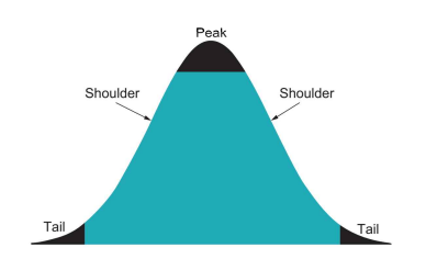
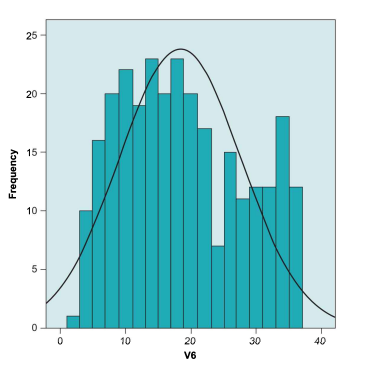
In this chapter we have seen how linear transformations can be used to change the scale of the data. A common transformation is from the original data to $z$-scores, which have a mean of 0 and a standard deviation of 1 . We can change the scale into any form through applying linear transformations. Adding and subtracting a constant shifts data over to the desired mean, and multiplying and dividing by a constant condenses or expands the scale. This shows that all scales and axes in statistics are arbitrary (Warne, 2014a). This will be an important issue in later chapters. Regardless of how we change the scale, a linear transformation will never change the shape of the histogram of a dataset (and, consequently, its skewness and kurtosis).
We can change the scale of a distribution by performing a linear transformation, which is the process of adding, subtracting, multiplying, or dividing the data by a constant. Adding and subtracting a constant will change the mean of a variable, but not its standard deviation or variance. Multiplying and dividing by a constant will change the mean, the standard deviation, and the variance of a dataset. Table $5.1$ shows how linear transformations change the values of models of central tendency and variability.
One special linear transformation is the $z$-score, the formula for which is Formula 5.7. All $z$-score values have a mean of 0 and a standard deviation of 1 . Putting datasets on a common scale permits comparisons across different units. Linear transformations, like the $z$-score, force the data to have the mean and standard deviation that we want. Yet, they do not change the shape of the distribution – only its scale. In fact, all scales are arbitrary, and we can use linear transformations to give our data any mean and standard deviation we choose. We can also convert data from $z$-scores to any other scale using the linear transformation equation in Formula $5.8$.
广义线性模型代写
统计代写|Generalized linear model代考广义线性模型代写|Linear Transformations
要执行线性变换,您需要获取一个数据集,然后将每个分数加、减、乘或除以相同的常数。(你可能记得在第 1 章中,常数是样本或总体中每个成员的相同分数。)执行线性变换在统计学中很常见。线性变换会改变数据,这意味着它们会影响从数据派生的模型——包括视觉模型和描述性统计。
线性变换允许我们将数据从一个尺度转换为更优选的尺度。例如,将以英寸为单位的测量值转换为厘米需要进行线性变换(乘以 2.54)。另一种常见的线性变换是将华氏温度转换为摄氏温度(需要减去 32,然后除以 1.8),反之亦然(需要乘以1.8然后添加 32 )。有时执行线性变换是为了使计算更容易,例如通过消除负数(通过添加一个常数使所有分数均为正数)或消除小数或分数(通过乘以一个常数)。正如您将在本章中看到的那样,对数据规模进行这些更改并不会从根本上改变分数的相对模式或许多统计分析的结果。
线性变换在统计中很常见,因此了解线性变换如何改变统计和数据非常重要。
线性变换对均值的影响。第 4 章展示了如何计算平均值(公式 4.2)和标准差(公式 4.7-4.9)。当将常数添加到数据中时,这些示例统计数据会发生一件有趣的事情。如果我们使用 Waite 等人。(2015) 数据并在每个人的年龄上加上一个常数 4,则结果如下:
求这些分数的平均值如下:
X¯喵喵 =22+23+24+25+27+27+28+28+29+35+37+39+4213 X¯喵喵 =38613=29.69
原始平均值(我们将其缩写为X¯原版 ) 为 25.69,如指导示例 4.1 所示。原始均值与新均值之差为4(29.69−25.69=4),它与添加到所有原始数据的常数相同。对于添加到数据集中每个分数的任何常数都是如此:X¯原版 + 持续的 =X¯新的
(公式 5.1)
统计代写|Generalized linear model代考广义线性模型代写|A Special Linear Transformation
社会科学中一种常见的线性变换是将数据转换为和-分数。一种和-score 是一种平均值为 0 且标准差为 1 的数据。将一组分数转换为和分数需要一个公式:
和一世=X一世−X¯sX
(公式 5.7)
在公式中5.7这X一世指变量的每个单独分数X,X¯是变量的样本均值X, 和sX是同一变量的标准差。这一世下标和一世表示数据集中的每个单独的分数都有自己的和-分数。
计算有两个步骤和-分数。第一步是在分子中,从每个分数中减去样本均值。(您可能会认为这是第 4 章中讨论过的偏差分数。)这一步将数据的平均值移动到 0 。第二步是除以数据的标准差。除以标准偏差会更改数据的比例,直到偏差精确等于 1。 指导实践5.1显示如何计算和- 真实数据的分数。
这个例子和- 指导实践中的分数计算5.1说明了几个原则和-分数。首先,注意原始分数低于原始平均值的每个人(即,X¯=25.69) 有一个负数和-score,每个原始分数高于原始平均值的个体都有一个正数和-分数。此外,当将原始分数与和-scores,很明显,分数最接近原始均值的受试者也有和- 最接近 0 的分数,这是和-分数。另一个原则是,单位和-scores 是标准差,意思是每个整数之间的差是一个标准差。最后,在这个例子中,原始数据中得分最低的人的得分也最低和-score——原始数据中得分最高的人也最高和-分数。事实上,对于原始数据和集合,受试者得分的排名顺序是相同的和-scores 因为线性变换(包括将原始分数转换为和-scores) 不会改变数据的形状或个人分数的排名。这些原则也适用于转换为的每个数据集和-分数。
有两个好处和-分数。首先是它们允许比较不同尺度的分数。与从事物理科学工作的研究人员不同,他们有明确的单位
测量(例如,米,克,磅),社会科学的研究人员和学生经常研究难以测量的变量(例如,紧张,婚姻中的沟通质量)。例如,对性别角色感兴趣的社会学家可以使用名为 Bem 性别角色清单 (Bem, 1974) 的测试来衡量研究中的受试者对传统男性或女性性别角色的认同程度。该测试有一个男性分量表和一个女性分量表,每个分量表的分数范围从 0 到 25 分,数字越高表明对男性或女性性别角色的认同越强。不过,心理学家可能会决定使用明尼苏达多相人格量表的男性气质和女性气质分量表(Butcher, Dahlstrom, Graham, Tellegen, & Kaemmer, 1989)来衡量性别角色。这些分量表的分数通常在 20 到 80 之间。即使两位研究人员都在测量相同的特征,他们的分数也没有可比性,因为量表是如此不同。但如果他们将数据转换为和-scores,则两项研究的分数具有可比性。
另一个好处是和-scores 允许我们对不同的变量进行比较。例如,人类学家可以发现她的一个研究对象有一个和- 分数+1.20在个人主义和和- 分数−0.43在文化传统主义的层面上。在这种情况下,她可以说这个人的个人主义水平高于他们的传统主义水平。这个例子表明,比较分数只需要分数在相同的范围内。因为和- 分数可以跨尺度和跨变量进行比较,它们就像一种“通用语言”,用于不同尺度和变量的数据。为此原因和- 分数有时被称为标准化分数。
统计代写|Generalized linear model代考广义线性模型代写|Linear Transformations and Scales
在本章中,我们看到了如何使用线性变换来改变数据的规模。一个常见的转换是从原始数据到和-scores,平均值为 0,标准差为 1。我们可以通过应用线性变换将比例更改为任何形式。添加和减去常数会将数据转移到所需的平均值,并且乘以和除以常数会压缩或扩展比例。这表明统计中的所有尺度和轴都是任意的(Warne,2014a)。这将是后面章节中的一个重要问题。不管我们如何改变尺度,线性变换永远不会改变数据集直方图的形状(因此,它的偏度和峰度)。
我们可以通过执行线性变换来改变分布的比例,线性变换是将数据加、减、乘或除以常数的过程。添加和减去一个常数会改变一个变量的平均值,但不会改变它的标准差或方差。乘以和除以常数将改变数据集的均值、标准差和方差。桌子5.1显示线性变换如何改变集中趋势和可变性模型的值。
一种特殊的线性变换是和-score,其公式为公式 5.7。全部和-score 值的平均值为 0 ,标准差为 1 。将数据集放在一个共同的尺度上可以跨不同的单位进行比较。线性变换,如和-score,强制数据具有我们想要的均值和标准差。然而,它们并没有改变分布的形状——只是改变了它的规模。事实上,所有尺度都是任意的,我们可以使用线性变换来为我们的数据提供我们选择的任何均值和标准差。我们还可以将数据从和- 使用公式中的线性变换方程得分到任何其他比例5.8.

统计代写请认准statistics-lab™. statistics-lab™为您的留学生涯保驾护航。
金融工程代写
金融工程是使用数学技术来解决金融问题。金融工程使用计算机科学、统计学、经济学和应用数学领域的工具和知识来解决当前的金融问题,以及设计新的和创新的金融产品。
非参数统计代写
非参数统计指的是一种统计方法,其中不假设数据来自于由少数参数决定的规定模型;这种模型的例子包括正态分布模型和线性回归模型。
广义线性模型代考
广义线性模型(GLM)归属统计学领域,是一种应用灵活的线性回归模型。该模型允许因变量的偏差分布有除了正态分布之外的其它分布。
术语 广义线性模型(GLM)通常是指给定连续和/或分类预测因素的连续响应变量的常规线性回归模型。它包括多元线性回归,以及方差分析和方差分析(仅含固定效应)。
有限元方法代写
有限元方法(FEM)是一种流行的方法,用于数值解决工程和数学建模中出现的微分方程。典型的问题领域包括结构分析、传热、流体流动、质量运输和电磁势等传统领域。
有限元是一种通用的数值方法,用于解决两个或三个空间变量的偏微分方程(即一些边界值问题)。为了解决一个问题,有限元将一个大系统细分为更小、更简单的部分,称为有限元。这是通过在空间维度上的特定空间离散化来实现的,它是通过构建对象的网格来实现的:用于求解的数值域,它有有限数量的点。边界值问题的有限元方法表述最终导致一个代数方程组。该方法在域上对未知函数进行逼近。[1] 然后将模拟这些有限元的简单方程组合成一个更大的方程系统,以模拟整个问题。然后,有限元通过变化微积分使相关的误差函数最小化来逼近一个解决方案。
tatistics-lab作为专业的留学生服务机构,多年来已为美国、英国、加拿大、澳洲等留学热门地的学生提供专业的学术服务,包括但不限于Essay代写,Assignment代写,Dissertation代写,Report代写,小组作业代写,Proposal代写,Paper代写,Presentation代写,计算机作业代写,论文修改和润色,网课代做,exam代考等等。写作范围涵盖高中,本科,研究生等海外留学全阶段,辐射金融,经济学,会计学,审计学,管理学等全球99%专业科目。写作团队既有专业英语母语作者,也有海外名校硕博留学生,每位写作老师都拥有过硬的语言能力,专业的学科背景和学术写作经验。我们承诺100%原创,100%专业,100%准时,100%满意。
随机分析代写
随机微积分是数学的一个分支,对随机过程进行操作。它允许为随机过程的积分定义一个关于随机过程的一致的积分理论。这个领域是由日本数学家伊藤清在第二次世界大战期间创建并开始的。
时间序列分析代写
随机过程,是依赖于参数的一组随机变量的全体,参数通常是时间。 随机变量是随机现象的数量表现,其时间序列是一组按照时间发生先后顺序进行排列的数据点序列。通常一组时间序列的时间间隔为一恒定值(如1秒,5分钟,12小时,7天,1年),因此时间序列可以作为离散时间数据进行分析处理。研究时间序列数据的意义在于现实中,往往需要研究某个事物其随时间发展变化的规律。这就需要通过研究该事物过去发展的历史记录,以得到其自身发展的规律。
回归分析代写
多元回归分析渐进(Multiple Regression Analysis Asymptotics)属于计量经济学领域,主要是一种数学上的统计分析方法,可以分析复杂情况下各影响因素的数学关系,在自然科学、社会和经济学等多个领域内应用广泛。
MATLAB代写
MATLAB 是一种用于技术计算的高性能语言。它将计算、可视化和编程集成在一个易于使用的环境中,其中问题和解决方案以熟悉的数学符号表示。典型用途包括:数学和计算算法开发建模、仿真和原型制作数据分析、探索和可视化科学和工程图形应用程序开发,包括图形用户界面构建MATLAB 是一个交互式系统,其基本数据元素是一个不需要维度的数组。这使您可以解决许多技术计算问题,尤其是那些具有矩阵和向量公式的问题,而只需用 C 或 Fortran 等标量非交互式语言编写程序所需的时间的一小部分。MATLAB 名称代表矩阵实验室。MATLAB 最初的编写目的是提供对由 LINPACK 和 EISPACK 项目开发的矩阵软件的轻松访问,这两个项目共同代表了矩阵计算软件的最新技术。MATLAB 经过多年的发展,得到了许多用户的投入。在大学环境中,它是数学、工程和科学入门和高级课程的标准教学工具。在工业领域,MATLAB 是高效研究、开发和分析的首选工具。MATLAB 具有一系列称为工具箱的特定于应用程序的解决方案。对于大多数 MATLAB 用户来说非常重要,工具箱允许您学习和应用专业技术。工具箱是 MATLAB 函数(M 文件)的综合集合,可扩展 MATLAB 环境以解决特定类别的问题。可用工具箱的领域包括信号处理、控制系统、神经网络、模糊逻辑、小波、仿真等。