如果你也在 怎样代写R这个学科遇到相关的难题,请随时右上角联系我们的24/7代写客服。
R是一个用于统计计算和图形的自由软件环境。
statistics-lab™ 为您的留学生涯保驾护航 在代写R方面已经树立了自己的口碑, 保证靠谱, 高质且原创的统计Statistics代写服务。我们的专家在代写R代写方面经验极为丰富,各种代写R相关的作业也就用不着说。
我们提供的R及其相关学科的代写,服务范围广, 其中包括但不限于:
- Statistical Inference 统计推断
- Statistical Computing 统计计算
- Advanced Probability Theory 高等楖率论
- Advanced Mathematical Statistics 高等数理统计学
- (Generalized) Linear Models 广义线性模型
- Statistical Machine Learning 统计机器学习
- Longitudinal Data Analysis 纵向数据分析
- Foundations of Data Science 数据科学基础
统计代写|R代写project|Numerical, graphical output
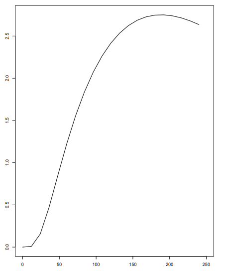
For ncase $=1$, the numerical output is the same as in Table $2.3$ and is not repeated here. Also, the graphical output is in Figs. $2.1$ for $V_{1}(x, t), C_{1}(x, t)$ and in Figs. $2.2$ for $V_{2}(x, t), C_{2}(x, t), q(t)$, and is not repeated here.
For ncase $=2$, the numerical output is in Table 4.1.
We can note the following details about this output.
- $21 t$ output points as the first dimension of the solution matrix out from lsodes as programmed in the main program of Listings 2.3, 4.1 (with nout $=21$ ).
- The solution matrix out returned by lsodes has 45 elements as a second dimension. The first element is the value of $t$. Elements 2 to 22 are $V_{1}(x, t)$ and elements 23 to 43 are $V_{2}(x, t)$ (for each of the 21 output points), elements 44,45 are $C_{1}(t), C_{2}(t)$.
- The solution is displayed for $t=0,240 / 20=48, \ldots, 240$ as programmed in Listings $2.3,4.1$ (every fourth value of $t$ is displayed as explained previously).
- ICs (1.1-4, 1.1-6), (1.2-4,1.2-6) are confirmed $(t=0)$.
- The solution varies with $t$ at $x=x_{u}=1$ in accordance with eq. (4.1).
- $C_{1}(t)$ initially (e.g., $t=48$ ) tracks the solution $V_{1}\left(x=x_{l}=0, t\right)$ as defined by $\mathrm{BC}$ (1.1-3) (at $x=0$ ) and the RHS of eq. (1.1-5). Later, (e.g., $t=240$ ), $C_{1}(t)$ and $V_{1}(x=0, t)$ reverse relative magnitudes.
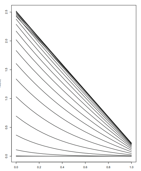
- $V_{2}\left(x=x_{l}=0, t\right)$ initially (e.g., $t=48$ ) tracks $C_{2}(t)$ according to $\mathrm{BC}(1.2-3)$ and the RHS of eq. (1.2-5). Later, (e.g., $t=240), C_{2}(t)$ and $V_{2}(x=0, t)$ reverse relative magnitudes.
- $V_{1}(x, t), V_{2}(x, t)$ for ncase $=1$ are substantially reduced for ncase $=2$, reflecting the effect of the vaccine. For example, at $t=240$, the reduction in $V_{2}(x, t)$ is indicated by a comparison of the output in Table $2.3$ and Table $4.1$ (ncase=2).
$\begin{array}{ccc}\text { Table } & 2.3 & \ t & x & \text { V2(t) } \ 240.0 & 0.0 & 4.382 e+01 \ 240.0 & 0.2 & 3.453 e+01 \ 240.0 & 0.4 & 2.603 e+01 \ 240.0 & 0.6 & 1.815 e+01 \ 240.0 & 0.8 & 1.072 \mathrm{e}+01 \ 240.0 & 1.0 & 3.547 \mathrm{e}+00 \ & & \ \text { Table } & 4.1 & \ t & x & \mathrm{~V} 2(\mathrm{t}) \ 240.0 & 0.0 & 2.426 \mathrm{e}+00 \ 240.0 & 0.2 & 2.000 \mathrm{e}+00 \ 240.0 & 0.4 & 1.565 \mathrm{e}+00 \ 240.0 & 0.6 & 1.122 \mathrm{e}+00 \ 240.0 & 0.8 & 6.750 \mathrm{e}-01 \ 240.0 & 1.0 & 2.252 \mathrm{e}-01\end{array}$ - The computational effort as indicated by ncall $=280$ is modest so that sodes [1] computed the solution to eqs. (1.1), (1.2), (4.1) efficiently.
统计代写|R代写project|ODE/PDE routine
The ODE/PDE routine pdelc called by lsodes in Listing $4.3$ includes the variation in $k_{r 2}$ with $t$ of eq. (4.2).
$#$
Variable kr2
if $($ ncase $==1){$
rate $\left.=\operatorname{kr} 2 * C 1^{\wedge} \mathrm{n} 2 ;\right}$
if $($ ncase $==2){$
rate $\left.=\mathrm{kr} 2 * \exp (-\mathrm{t} / \operatorname{tau}) * \mathrm{Cl}{ }^{\wedge} \mathrm{n} 2 ;\right}$
$#$
ODEs
$\mathrm{C} 1 \mathrm{t}=-\mathrm{k} 1] *(\mathrm{C} 1-\mathrm{V} 1[1])$;
$\mathrm{C} 2 \mathrm{t}=-\mathrm{k} 2 l *(\mathrm{C} 2-\mathrm{V} 2[1])+$ rate;
Listing 4.4 Variation of $k_{r 2}$ in ODE/PDE routine pde1c
rate is used in eq. $(1.2-5)\left(\mathrm{C} 2 \mathrm{t}=\frac{d C_{2}(t)}{d t}\right)$.
Two cases are programmed:
- ncase $=1$ is the base case of Listings $2.3,4.3$ for constant $k_{r 2}$.
- ncase $=2$ is the time variable case of eq. (4.2), that is, $k_{r 2}(t)$ decreases exponentially in $t$ to reflect the effect of the therapeutic. $t$ is the first argument of the routine, pdel $\mathrm{c}=$ function $(t, u$, parm). $\tau$ is set in Listing 4.3.
统计代写|R代写project|Numerical, graphical output
For ncase $=1$, the numerical output is the same as in Table $2.3$ and is not repeated here. Also, the graphical output is in Figs. $2.1$ for $V_{1}(x, t), C_{1}(x, t)$ and in Figs. $2.2$ for $V_{2}(x, t), C_{2}(x, t), q(t)$, and is not repeated here.
For ncase $=2$, the numerical output is in Table 4.2.
We can note the following details about this output.
- $21 t$ output points as the first dimension of the solution matrix out from lsodes as programmed in the main program of Listings $2.3,4.3$ (with nout =21).
- The solution matrix out returned by lsodes has 45 elements as a second dimension. The first element is the value of $t$. Elements 2 to 22 are $V_{1}(x, t)$ and elements 23 to 43 are $V_{2}(x, t)$ (for each of the 21 output points), elements 44,45 are $C_{1}(t), C_{2}(t)$.
- The solution is displayed for $t=0,240 / 20=48, \ldots, 240$ as programmed in Listings $2.3,4.3$ (every fourth value of $t$ is displayed as explained previously).
- ICs (1.1-4, 1.1-6), (1.2-4, 1.2-6) are confirmed $(t=0)$.
The solution varies with $t$ in accordance with eq. (4.2). Since rate in eq. (4.2) affects only $V_{2}(x, t), C_{2}(t)$ through eq. (1.2-5), $V_{1}(x, t), C_{1}(t)$ are unchanged for ncase $=1,2$ (compare Tables $2.3$ and 4.2).
$C_{1}(t)$ tracks the solution as defined by $\mathrm{BC}(1.1-3)$ (at $\left.x=0\right)$ and the RHS of eq. (1.1-5).
$V_{2}\left(x=x_{1}=0, t\right)$ tracks $C_{2}(t)$ according to $\mathrm{BC}(1.2-3)$.
$V_{2}(x, t)$ for ncase $=1$ is substantially reduced for ncase $=2$, reflecting the effect of the therapeutic. For example, at $t=240$, the reduction in $V_{2}(x, t)$ is indicated by a comparison of the output in Table $2.3$ and Table $4.2($ ncase $=2$ ).
R代考
统计代写|R代写project|Numerical, graphical output
对于 ncase=1,数值输出与表中相同2.3并且在此不再赘述。此外,图形输出在图 1 和图 3 中。2.1为了在1(X,吨),C1(X,吨)并在无花果。2.2为了在2(X,吨),C2(X,吨),q(吨), 此处不再赘述。
对于 ncase=2,数值输出如表 4.1 所示。
我们可以注意到有关此输出的以下详细信息。
- 21吨输出点作为从 lsodes 输出的解矩阵的第一维,如清单 2.3、4.1 的主程序中编程的那样(没有=21 ).
- lsodes 返回的解矩阵 out 有 45 个元素作为第二维。第一个元素是值吨. 元素 2 到 22 是在1(X,吨)元素 23 到 43 是在2(X,吨)(对于 21 个输出点中的每一个),元素 44,45 是C1(吨),C2(吨).
- 解决方案显示为吨=0,240/20=48,…,240如清单中的程序2.3,4.1(每四个值吨显示如前所述)。
- IC (1.1-4, 1.1-6), (1.2-4,1.2-6) 已确认(吨=0).
- 解决方案因吨在X=X在=1根据等式。(4.1)。
- C1(吨)最初(例如,吨=48) 跟踪解决方案在1(X=Xl=0,吨)定义为乙C(1.1-3) (在X=0) 和等式的 RHS。(1.1-5)。后来,(例如,吨=240 ), C1(吨)和在1(X=0,吨)反向相对大小。
- 在2(X=Xl=0,吨)最初(例如,吨=48) 轨道C2(吨)根据乙C(1.2−3)和 eq 的 RHS。(1.2-5)。后来,(例如,吨=240),C2(吨)和在2(X=0,吨)反向相对大小。
- 在1(X,吨),在2(X,吨)对于 ncase=1ncase 大大减少=2,反映疫苗的效果。例如,在吨=240,减少在2(X,吨)由表中的输出比较表示2.3和表4.1(ncase=2)。
桌子 2.3 吨X V2(t) 240.00.04.382和+01 240.00.23.453和+01 240.00.42.603和+01 240.00.61.815和+01 240.00.81.072和+01 240.01.03.547和+00 桌子 4.1 吨X 在2(吨) 240.00.02.426和+00 240.00.22.000和+00 240.00.41.565和+00 240.00.61.122和+00 240.00.86.750和−01 240.01.02.252和−01 - ncall 表示的计算量=280是适度的,因此 sodes [1] 计算出 eqs 的解。(1.1), (1.2), (4.1) 有效。
统计代写|R代写project|ODE/PDE routine
清单中 lsodes 调用的 ODE/PDE 例程 pdelc4.3包括变化ķr2和吨当量 (4.2)。
##
变量 kr2
如果(案例==1){$ 费率 $\left.=\operatorname{kr} 2 * C 1^{\wedge} \mathrm{n} 2 ;\right}==1){$ 费率 $\left.=\operatorname{kr} 2 * C 1^{\wedge} \mathrm{n} 2 ;\right}
如果(案例==2){$ rate $\left.=\mathrm{kr} 2 * \exp (-\mathrm{t} / \operatorname{tau}) * \mathrm{Cl}{ }^{\wedge} \mathrm {n} 2 ;\右}==2){$ rate $\left.=\mathrm{kr} 2 * \exp (-\mathrm{t} / \operatorname{tau}) * \mathrm{Cl}{ }^{\wedge} \mathrm {n} 2 ;\右}
##
常微分方程
C1吨=−ķ1]∗(C1−在1[1]);
C2吨=−ķ2l∗(C2−在2[1])+速度;
清单 4.4 的变体ķr2在 ODE/PDE 例程中,方程中使用 pde1c
速率。(1.2−5)(C2吨=dC2(吨)d吨).
编程了两种情况:
- 案例=1是列表的基本情况2.3,4.3为常数ķr2.
- 案例=2是 eq 的时间变量情况。(4.2),即ķr2(吨)呈指数下降吨反映治疗效果。吨是例程的第一个参数,pdelC=功能(吨,在, 参数)。τ在清单 4.3 中设置。
统计代写|R代写project|Numerical, graphical output
对于 ncase=1,数值输出与表中相同2.3并且在此不再赘述。此外,图形输出在图 1 和图 3 中。2.1为了在1(X,吨),C1(X,吨)并在无花果。2.2为了在2(X,吨),C2(X,吨),q(吨), 此处不再赘述。
对于 ncase=2,数值输出见表 4.2。
我们可以注意到有关此输出的以下详细信息。
- 21吨输出点作为解决方案矩阵的第一维从 lsodes 输出,如清单主程序中编程的那样2.3,4.3(没有= 21)。
- lsodes 返回的解矩阵 out 有 45 个元素作为第二维。第一个元素是值吨. 元素 2 到 22 是在1(X,吨)元素 23 到 43 是在2(X,吨)(对于 21 个输出点中的每一个),元素 44,45 是C1(吨),C2(吨).
- 解决方案显示为吨=0,240/20=48,…,240如清单中的程序2.3,4.3(每四个值吨显示如前所述)。
- IC (1.1-4, 1.1-6), (1.2-4, 1.2-6) 已确认(吨=0).
解决方案因吨根据等式。(4.2)。由于方程中的速率。(4.2) 仅影响在2(X,吨),C2(吨)通过等式。(1.2-5),在1(X,吨),C1(吨)ncase 不变=1,2(比较表2.3和 4.2)。
C1(吨)跟踪定义的解决方案乙C(1.1−3)(在X=0)和 eq 的 RHS。(1.1-5)。
在2(X=X1=0,吨)轨道C2(吨)根据乙C(1.2−3).
在2(X,吨)对于 ncase=1ncase 大大减少=2,反映治疗效果。例如,在吨=240,减少在2(X,吨)由表中的输出比较表示2.3和表4.2(案例=2 ).

统计代写请认准statistics-lab™. statistics-lab™为您的留学生涯保驾护航。
金融工程代写
金融工程是使用数学技术来解决金融问题。金融工程使用计算机科学、统计学、经济学和应用数学领域的工具和知识来解决当前的金融问题,以及设计新的和创新的金融产品。
非参数统计代写
非参数统计指的是一种统计方法,其中不假设数据来自于由少数参数决定的规定模型;这种模型的例子包括正态分布模型和线性回归模型。
广义线性模型代考
广义线性模型(GLM)归属统计学领域,是一种应用灵活的线性回归模型。该模型允许因变量的偏差分布有除了正态分布之外的其它分布。
术语 广义线性模型(GLM)通常是指给定连续和/或分类预测因素的连续响应变量的常规线性回归模型。它包括多元线性回归,以及方差分析和方差分析(仅含固定效应)。
有限元方法代写
有限元方法(FEM)是一种流行的方法,用于数值解决工程和数学建模中出现的微分方程。典型的问题领域包括结构分析、传热、流体流动、质量运输和电磁势等传统领域。
有限元是一种通用的数值方法,用于解决两个或三个空间变量的偏微分方程(即一些边界值问题)。为了解决一个问题,有限元将一个大系统细分为更小、更简单的部分,称为有限元。这是通过在空间维度上的特定空间离散化来实现的,它是通过构建对象的网格来实现的:用于求解的数值域,它有有限数量的点。边界值问题的有限元方法表述最终导致一个代数方程组。该方法在域上对未知函数进行逼近。[1] 然后将模拟这些有限元的简单方程组合成一个更大的方程系统,以模拟整个问题。然后,有限元通过变化微积分使相关的误差函数最小化来逼近一个解决方案。
tatistics-lab作为专业的留学生服务机构,多年来已为美国、英国、加拿大、澳洲等留学热门地的学生提供专业的学术服务,包括但不限于Essay代写,Assignment代写,Dissertation代写,Report代写,小组作业代写,Proposal代写,Paper代写,Presentation代写,计算机作业代写,论文修改和润色,网课代做,exam代考等等。写作范围涵盖高中,本科,研究生等海外留学全阶段,辐射金融,经济学,会计学,审计学,管理学等全球99%专业科目。写作团队既有专业英语母语作者,也有海外名校硕博留学生,每位写作老师都拥有过硬的语言能力,专业的学科背景和学术写作经验。我们承诺100%原创,100%专业,100%准时,100%满意。
随机分析代写
随机微积分是数学的一个分支,对随机过程进行操作。它允许为随机过程的积分定义一个关于随机过程的一致的积分理论。这个领域是由日本数学家伊藤清在第二次世界大战期间创建并开始的。
时间序列分析代写
随机过程,是依赖于参数的一组随机变量的全体,参数通常是时间。 随机变量是随机现象的数量表现,其时间序列是一组按照时间发生先后顺序进行排列的数据点序列。通常一组时间序列的时间间隔为一恒定值(如1秒,5分钟,12小时,7天,1年),因此时间序列可以作为离散时间数据进行分析处理。研究时间序列数据的意义在于现实中,往往需要研究某个事物其随时间发展变化的规律。这就需要通过研究该事物过去发展的历史记录,以得到其自身发展的规律。
回归分析代写
多元回归分析渐进(Multiple Regression Analysis Asymptotics)属于计量经济学领域,主要是一种数学上的统计分析方法,可以分析复杂情况下各影响因素的数学关系,在自然科学、社会和经济学等多个领域内应用广泛。
MATLAB代写
MATLAB 是一种用于技术计算的高性能语言。它将计算、可视化和编程集成在一个易于使用的环境中,其中问题和解决方案以熟悉的数学符号表示。典型用途包括:数学和计算算法开发建模、仿真和原型制作数据分析、探索和可视化科学和工程图形应用程序开发,包括图形用户界面构建MATLAB 是一个交互式系统,其基本数据元素是一个不需要维度的数组。这使您可以解决许多技术计算问题,尤其是那些具有矩阵和向量公式的问题,而只需用 C 或 Fortran 等标量非交互式语言编写程序所需的时间的一小部分。MATLAB 名称代表矩阵实验室。MATLAB 最初的编写目的是提供对由 LINPACK 和 EISPACK 项目开发的矩阵软件的轻松访问,这两个项目共同代表了矩阵计算软件的最新技术。MATLAB 经过多年的发展,得到了许多用户的投入。在大学环境中,它是数学、工程和科学入门和高级课程的标准教学工具。在工业领域,MATLAB 是高效研究、开发和分析的首选工具。MATLAB 具有一系列称为工具箱的特定于应用程序的解决方案。对于大多数 MATLAB 用户来说非常重要,工具箱允许您学习和应用专业技术。工具箱是 MATLAB 函数(M 文件)的综合集合,可扩展 MATLAB 环境以解决特定类别的问题。可用工具箱的领域包括信号处理、控制系统、神经网络、模糊逻辑、小波、仿真等。