如果你也在 怎样代写机器学习machine learning这个学科遇到相关的难题,请随时右上角联系我们的24/7代写客服。
机器学习(ML)是人工智能(AI)的一种类型,它允许软件应用程序在预测结果时变得更加准确,而无需明确编程。机器学习算法使用历史数据作为输入来预测新的输出值。
statistics-lab™ 为您的留学生涯保驾护航 在代写机器学习machine learning方面已经树立了自己的口碑, 保证靠谱, 高质且原创的统计Statistics代写服务。我们的专家在代写机器学习machine learning代写方面经验极为丰富,各种代写机器学习machine learning相关的作业也就用不着说。
我们提供的机器学习machine learning及其相关学科的代写,服务范围广, 其中包括但不限于:
- Statistical Inference 统计推断
- Statistical Computing 统计计算
- Advanced Probability Theory 高等概率论
- Advanced Mathematical Statistics 高等数理统计学
- (Generalized) Linear Models 广义线性模型
- Statistical Machine Learning 统计机器学习
- Longitudinal Data Analysis 纵向数据分析
- Foundations of Data Science 数据科学基础
计算机代写|机器学习代写machine learning代考|Convex Optimization
When building a model in the context of machine learning, we often seek optimal model parameters $\boldsymbol{\theta}$, in the sense where they maximize the prior probability (or probability density) of predicting observed data. Here, we denote by $\tilde{f}(\theta)$ the target function we want to maximize. Optimal parameter values $\theta^{}$ are those that maximize the function $\hat{f}(\boldsymbol{\theta})$. $$ \boldsymbol{\theta}^{}=\underset{\boldsymbol{\theta}}{\arg \max } \tilde{f}(\boldsymbol{\theta}) .
$$
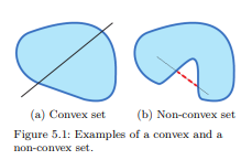
With a small caveat that will be covered below, convex optimization methods can be employed for the maximization task in equation 5.1. The key aspect of convex optimization methods is that, under certain conditions, they are guaranteed to reach optimal values for convex functions. Figure $5.1$ presents examples of convex and non-convex sets. For a set to be convex, you must be able to link any two points belonging to it without being outside of this set. Figure 5.1b presents a case where this property is not satisfied. For a convex function, the segment linking any pair of its points lies above or is equal to the function. Conversely, for a concave function, the opposite holds: the segment linking any pair of points lies below or is equal to the function. A concave function can be transformed into a convex one by taking the negative of it. Therefore, a maximization problem formulated as a concave optimization can be formulated in terms of a convex optimization following
$$
\boldsymbol{\theta}^{}=\underbrace{\underset{\theta}{\arg \max } \tilde{f}(\boldsymbol{\theta})}{\text {Concave optimization }} \equiv \underbrace{\arg \min -\tilde{f}(\boldsymbol{\theta})}{\text {Convex optimization }}
$$
In this chapter, we refer to convex optimization even if we are interested in maximizing a concave function, rather than minimizing a convex one. This choice is justified by the prevalence of convex optimization in the literature. Moreover, note that for several machine learning methods, we seek $\theta^{}$ based on a minimization problem where $-\tilde{f}(\boldsymbol{\theta})$ is a function of the difference between observed values and those predicted by a model. Figure $5.2$ presents examples of convex/concave and non-convex/non-concave functions. Nonconvex/non-concave functions such as the one in figure $5.2 \mathrm{~b}$ may have several local optima. Many functions of practical interest are non-convex/non-concave. As we will see in this chapter, convex optimization methods can also be employed for non-convex/nonconcave functions given that we choose a proper starting location. This chapter presents the gradient ascent and Newton-Raphson methods, as well as practical tools to be employed with them. For full-depth details regarding optimization methods, the reader should refer to dedicated textbooks. 1
计算机代写|机器学习代写machine learning代考|Gradient Ascent
A gradient is a vector containing the partial derivatives of a function with respect to its variables. For a continuous function, the maximum is located at the point where its gradient equals zero. Gradient ascent is based on the principle that as long as we move in the direction of the gradient, we are moving toward a maximum. For the unidimensional case, we choose to move to a new position by a scaling factor $\lambda$ times the derivative estimated at $\theta_{\text {old }}$,
$$
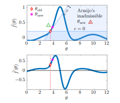
\theta_{\text {new }}=\theta_{\text {old }}+\underbrace{\lambda \cdot \tilde{f}^{\prime}\left(\theta_{\text {old }}\right)}{d} . $$ A common practice for setting $\lambda$ is to employ bachtracking line search where a new position is accepted if the Armijo rule ${ }^{2}$ is satisfied so that $$ \tilde{f}\left(\theta{\text {new }}\right) \geq \tilde{f}\left(\theta_{\text {old }}\right)+c \cdot d \tilde{f}^{\prime}\left(\theta_{\text {old }}\right) \text {, with } c \in(0,1) \text {. }
$$
Figure $5.3$ presents a comparison of the application of equation $5.2$ with the two extreme cases, $c=0$ and $c=1$. For $c=1, \theta_{\text {new }}$ is only accepted if $f\left(\theta_{\text {new }}\right)$ lies above the plane defined by the tangent at $\theta_{\text {old }}$. For $c=0, \theta_{\text {new }}$ is only accepted if $\tilde{f}\left(\theta_{\text {new }}\right)>\tilde{f}\left(\theta_{\text {old }}\right)$. The larger $c$ is, the stricter is the Armijo rule for ensuring that sufficient progress is made by the current step. With backtracking line search, we start from an initial value of $\lambda_{0}$ and reduce it until equation $5.2$ is satisfied. Algorithm 1 presents a minimal version of the gradient ascent with backtracking line search.
计算机代写|机器学习代写machine learning代考|Newton-Raphson
The Newton-Raphson method allows us to adaptively scale the search direction vector using the second-order derivative $\tilde{f}^{\prime \prime}(\theta)$. Knowing that the maximum of a function corresponds to the point where the gradient is zero, $\tilde{f}^{\prime}(\theta)=0$, we can find this maximum by formulating a linearized gradient equation using the second-order derivative of $\tilde{f}(\theta)$ and then set it equal to zero. The analytic formulation for the linearized gradient function (see \$3.4.2) approximated at the current location $\theta_{\text {old }}$ is
$$
\tilde{f}^{\prime}(\theta) \approx \tilde{f}^{\prime \prime}\left(\theta_{\text {old }}\right) \cdot\left(\theta-\theta_{\text {old }}\right)+\tilde{f}^{\prime \prime}\left(\theta_{\text {old }}\right)
$$
We can estimate $\theta_{\text {new }}$ by setting equation $5.3$ equal to zero, and then by solving for $\theta$, we obtain
$$
\theta_{\text {new }}=\theta_{\text {old }}-\frac{\tilde{f}^{\prime}\left(\theta_{\text {old }}\right)}{f^{\prime \prime}\left(\theta_{\text {old }}\right)}
$$
Let us consider the case where we want to find the maximum of a quadratic function (i.e., $\propto x^{2}$ ), as illustrated in figure 5.7. In the case of a quadratic function, the algorithm converges to the exact solution in one iteration, no matter the starting point, because the gradient of a quadratic function is exactly described by the linear function in equation $5.3$.
Algorithm 2 presents a minimal version of the Newton-Raphson method with backtracking line search. Note that at line 6 , there is again a scaling factor $\lambda$, which is employed because the NewtonRaphson method is exact only for quadratic functions. For more general non-convex/non-concave functions, the linearized gradient is an approximation such that a value of $\lambda=1$ will not always lead to a $\theta_{\text {new }}$ satisfying the Armijo rule in equation 5.2.
Figure $5.8$ presents the application of algorithm 2 to a nonconvex/non-concave function with an initial value $\theta_{0}=3.5$ and a scaling factor $\lambda_{0}=1$. For each loop, the pink solid line represents the linearized gradient function formulated in equation 5.3. Notice how, for the first two iterations, the second derivative $f^{\prime \prime}(\theta)>0$. Having a positive second derivative indicates that the linearization of $\tilde{f}^{\prime}(\theta)$ equals zero for a minimum rather than for a maximum. One simple option in this situation is to define $\lambda=-\lambda$ in order to ensure that the next slep moves in the same dirextion as the gradient. The convergence with Newton-Raphson is typically faster than with gradient ascent.
机器学习代考
计算机代写|机器学习代写machine learning代考|Convex Optimization
在机器学习的背景下构建模型时,我们经常寻求最优的模型参数θ,在它们最大化预测观察数据的先验概率(或概率密度)的意义上。在这里,我们表示F~(θ)我们想要最大化的目标函数。最佳参数值θ是最大化功能的那些F^(θ).
θ=参数最大限度θF~(θ).
有一点将在下面介绍,凸优化方法可以用于方程 5.1 中的最大化任务。凸优化方法的关键在于,在某些条件下,它们保证达到凸函数的最优值。数字5.1给出了凸集和非凸集的例子。对于一个凸集,您必须能够链接属于它的任何两个点,而不会超出该集。图 5.1b 展示了一个不满足此属性的情况。对于凸函数,连接其任意一对点的线段位于该函数之上或等于该函数。相反,对于凹函数,相反的情况成立:连接任何一对点的线段位于该函数的下方或等于该函数。一个凹函数可以通过取负数转换为一个凸函数。因此,一个被表述为凹优化的最大化问题可以被表述为以下的凸优化
θ=参数最大限度θF~(θ)⏟凹优化 ≡参数分钟−F~(θ)⏟凸优化
在本章中,即使我们对最大化凹函数而不是最小化凸函数感兴趣,我们也会提到凸优化。文献中凸优化的普遍性证明了这种选择是合理的。此外,请注意,对于几种机器学习方法,我们寻求θ基于最小化问题,其中−F~(θ)是观测值与模型预测值之间差异的函数。数字5.2给出了凸/凹和非凸/非凹函数的例子。非凸/非凹函数,如图所示5.2 b可能有几个局部最优值。许多实际感兴趣的函数是非凸/非凹的。正如我们将在本章中看到的,如果我们选择了合适的起始位置,凸优化方法也可以用于非凸/非凹函数。本章介绍梯度上升法和 Newton-Raphson 方法,以及与它们一起使用的实用工具。有关优化方法的详细信息,读者应参考专门的教科书。1
计算机代写|机器学习代写machine learning代考|Gradient Ascent
梯度是包含函数相对于其变量的偏导数的向量。对于连续函数,最大值位于其梯度为零的点。梯度上升是基于这样的原理,只要我们沿着梯度的方向移动,我们就会朝着一个最大值移动。对于一维情况,我们选择按比例因子移动到新位置λ乘以估计的导数θ老的 ,
θ新的 =θ老的 +λ⋅F~′(θ老的 )⏟d.设置的常见做法λ是采用 bachtracking 线搜索,如果 Armijo 规则接受新位置2满足,使得
F~(θ新的 )≥F~(θ老的 )+C⋅dF~′(θ老的 ), 和 C∈(0,1).
数字5.3比较了方程的应用5.2在两种极端情况下,C=0和C=1. 为了C=1,θ新的 仅在以下情况下被接受F(θ新的 )位于由切线定义的平面之上θ老的 . 为了C=0,θ新的 仅在以下情况下被接受F~(θ新的 )>F~(θ老的 ). 较大的C也就是说,更严格的是确保当前步骤取得足够进展的 Armijo 规则。通过回溯线搜索,我们从初始值开始λ0并减少它直到方程5.2很满意。算法 1 提出了带有回溯线搜索的梯度上升的最小版本。
计算机代写|机器学习代写machine learning代考|Newton-Raphson
Newton-Raphson 方法允许我们使用二阶导数自适应地缩放搜索方向向量F~′′(θ). 知道函数的最大值对应于梯度为零的点,F~′(θ)=0,我们可以通过使用的二阶导数制定线性梯度方程来找到这个最大值F~(θ)然后将其设置为零。在当前位置近似的线性化梯度函数的解析公式(见$ 3.4.2)θ老的 是
F~′(θ)≈F~′′(θ老的 )⋅(θ−θ老的 )+F~′′(θ老的 )
我们可以估计θ新的 通过设置方程5.3等于零,然后通过求解θ, 我们获得
θ新的 =θ老的 −F~′(θ老的 )F′′(θ老的 )
让我们考虑一下我们想要找到二次函数的最大值的情况(即,∝X2),如图 5.7 所示。在二次函数的情况下,算法在一次迭代中收敛到精确解,无论起点如何,因为二次函数的梯度精确地由方程中的线性函数描述5.3.
算法 2 提供了带有回溯线搜索的 Newton-Raphson 方法的最小版本。请注意,在第 6 行,还有一个比例因子λ,这是因为 NewtonRaphson 方法仅适用于二次函数。对于更一般的非凸/非凹函数,线性化梯度是一个近似值,使得λ=1不会总是导致θ新的 满足方程 5.2 中的 Armijo 规则。
数字5.8将算法 2 应用于具有初始值的非凸/非凹函数θ0=3.5和比例因子λ0=1. 对于每个循环,粉红色实线表示方程 5.3 中公式化的线性梯度函数。请注意,对于前两次迭代,二阶导数F′′(θ)>0. 具有正二阶导数表示线性化F~′(θ)最小值等于 0,而不是最大值。在这种情况下,一个简单的选择是定义λ=−λ为了确保下一个 slep 在与梯度相同的方向上移动。与 Newton-Raphson 的收敛通常比梯度上升更快。

统计代写请认准statistics-lab™. statistics-lab™为您的留学生涯保驾护航。
金融工程代写
金融工程是使用数学技术来解决金融问题。金融工程使用计算机科学、统计学、经济学和应用数学领域的工具和知识来解决当前的金融问题,以及设计新的和创新的金融产品。
非参数统计代写
非参数统计指的是一种统计方法,其中不假设数据来自于由少数参数决定的规定模型;这种模型的例子包括正态分布模型和线性回归模型。
广义线性模型代考
广义线性模型(GLM)归属统计学领域,是一种应用灵活的线性回归模型。该模型允许因变量的偏差分布有除了正态分布之外的其它分布。
术语 广义线性模型(GLM)通常是指给定连续和/或分类预测因素的连续响应变量的常规线性回归模型。它包括多元线性回归,以及方差分析和方差分析(仅含固定效应)。
有限元方法代写
有限元方法(FEM)是一种流行的方法,用于数值解决工程和数学建模中出现的微分方程。典型的问题领域包括结构分析、传热、流体流动、质量运输和电磁势等传统领域。
有限元是一种通用的数值方法,用于解决两个或三个空间变量的偏微分方程(即一些边界值问题)。为了解决一个问题,有限元将一个大系统细分为更小、更简单的部分,称为有限元。这是通过在空间维度上的特定空间离散化来实现的,它是通过构建对象的网格来实现的:用于求解的数值域,它有有限数量的点。边界值问题的有限元方法表述最终导致一个代数方程组。该方法在域上对未知函数进行逼近。[1] 然后将模拟这些有限元的简单方程组合成一个更大的方程系统,以模拟整个问题。然后,有限元通过变化微积分使相关的误差函数最小化来逼近一个解决方案。
tatistics-lab作为专业的留学生服务机构,多年来已为美国、英国、加拿大、澳洲等留学热门地的学生提供专业的学术服务,包括但不限于Essay代写,Assignment代写,Dissertation代写,Report代写,小组作业代写,Proposal代写,Paper代写,Presentation代写,计算机作业代写,论文修改和润色,网课代做,exam代考等等。写作范围涵盖高中,本科,研究生等海外留学全阶段,辐射金融,经济学,会计学,审计学,管理学等全球99%专业科目。写作团队既有专业英语母语作者,也有海外名校硕博留学生,每位写作老师都拥有过硬的语言能力,专业的学科背景和学术写作经验。我们承诺100%原创,100%专业,100%准时,100%满意。
随机分析代写
随机微积分是数学的一个分支,对随机过程进行操作。它允许为随机过程的积分定义一个关于随机过程的一致的积分理论。这个领域是由日本数学家伊藤清在第二次世界大战期间创建并开始的。
时间序列分析代写
随机过程,是依赖于参数的一组随机变量的全体,参数通常是时间。 随机变量是随机现象的数量表现,其时间序列是一组按照时间发生先后顺序进行排列的数据点序列。通常一组时间序列的时间间隔为一恒定值(如1秒,5分钟,12小时,7天,1年),因此时间序列可以作为离散时间数据进行分析处理。研究时间序列数据的意义在于现实中,往往需要研究某个事物其随时间发展变化的规律。这就需要通过研究该事物过去发展的历史记录,以得到其自身发展的规律。
回归分析代写
多元回归分析渐进(Multiple Regression Analysis Asymptotics)属于计量经济学领域,主要是一种数学上的统计分析方法,可以分析复杂情况下各影响因素的数学关系,在自然科学、社会和经济学等多个领域内应用广泛。
MATLAB代写
MATLAB 是一种用于技术计算的高性能语言。它将计算、可视化和编程集成在一个易于使用的环境中,其中问题和解决方案以熟悉的数学符号表示。典型用途包括:数学和计算算法开发建模、仿真和原型制作数据分析、探索和可视化科学和工程图形应用程序开发,包括图形用户界面构建MATLAB 是一个交互式系统,其基本数据元素是一个不需要维度的数组。这使您可以解决许多技术计算问题,尤其是那些具有矩阵和向量公式的问题,而只需用 C 或 Fortran 等标量非交互式语言编写程序所需的时间的一小部分。MATLAB 名称代表矩阵实验室。MATLAB 最初的编写目的是提供对由 LINPACK 和 EISPACK 项目开发的矩阵软件的轻松访问,这两个项目共同代表了矩阵计算软件的最新技术。MATLAB 经过多年的发展,得到了许多用户的投入。在大学环境中,它是数学、工程和科学入门和高级课程的标准教学工具。在工业领域,MATLAB 是高效研究、开发和分析的首选工具。MATLAB 具有一系列称为工具箱的特定于应用程序的解决方案。对于大多数 MATLAB 用户来说非常重要,工具箱允许您学习和应用专业技术。工具箱是 MATLAB 函数(M 文件)的综合集合,可扩展 MATLAB 环境以解决特定类别的问题。可用工具箱的领域包括信号处理、控制系统、神经网络、模糊逻辑、小波、仿真等。