如果你也在 怎样代写机器学习machine learning这个学科遇到相关的难题,请随时右上角联系我们的24/7代写客服。
机器学习(ML)是人工智能(AI)的一种类型,它允许软件应用程序在预测结果时变得更加准确,而无需明确编程。机器学习算法使用历史数据作为输入来预测新的输出值。
statistics-lab™ 为您的留学生涯保驾护航 在代写机器学习machine learning方面已经树立了自己的口碑, 保证靠谱, 高质且原创的统计Statistics代写服务。我们的专家在代写机器学习machine learning代写方面经验极为丰富,各种代写机器学习machine learning相关的作业也就用不着说。
我们提供的机器学习machine learning及其相关学科的代写,服务范围广, 其中包括但不限于:
- Statistical Inference 统计推断
- Statistical Computing 统计计算
- Advanced Probability Theory 高等概率论
- Advanced Mathematical Statistics 高等数理统计学
- (Generalized) Linear Models 广义线性模型
- Statistical Machine Learning 统计机器学习
- Longitudinal Data Analysis 纵向数据分析
- Foundations of Data Science 数据科学基础
计算机代写|机器学习代写machine learning代考|Univariate Normal
The probability density function (PDF) for a Normal random variable is defined over the real numbers $x \in \mathbb{R} . X \sim \mathcal{N}\left(x ; \mu, \sigma^{2}\right)$ is parameterized by its mean $\mu$ and variance $\sigma^{2}$, so its PDF is
$$
f_{X}(x)=\mathcal{N}\left(x ; \mu, \sigma^{2}\right)=\frac{1}{\sqrt{2 \pi} \sigma} \exp \left(-\frac{1}{2}\left(\frac{x-\mu}{\sigma}\right)^{2}\right)
$$
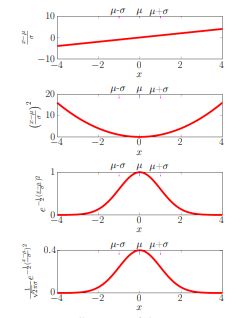
Figure 4.1 presents an example of PDF and cumulative distribution function (CDF) with parameters $\mu=0$ and $\sigma=1$. The mode that is, the most likely value-corresponds to the mean. Changing the mean $\mu$ causes a translation of the distribution. Increasing the standard deviation $\sigma$ causes a proportional increase in the PDF’s dispersion. The Normal CDF is presented in figure 4.1b. Its formulation is obtained through integration, where the integral can
be formulated using the error function erf(-),
$$
\begin{aligned}
F_{X}(x) &=\int_{-\infty}^{x} \frac{1}{\sqrt{2 \pi} \sigma} \exp \left(-\frac{1}{2}\left(\frac{x^{\prime}-\mu}{\sigma}\right)^{2}\right) d x^{\prime} \
&=\frac{1}{2}\left(1+\operatorname{erf}\left(\frac{x-\mu}{\sigma \sqrt{2}}\right)\right)
\end{aligned}
$$
Figure $4.2$ illustrates the successive steps taken to construct the univariate Normal PDF. Within the innermost parenthesis of the PDF formulation is a linear function $\frac{x-\mu}{\sigma}$, which centers $x$ on the mean $\mu$ and normalizes it with the standard deviation $\sigma$. This first term is then squared, leading to a positive number over all its domain except at the mean, where it is equal to zero. Taking the negative exponential of this second term leads to a bell-shaped curve, where the value equals one $(\exp (0)=1)$ at the mean $x=\mu$ and where there are inflexion points at $\mu \pm \sigma$. At this step, the curve is proportional to the final Normal PDF. Only the normalization constant is missing to ensure that $\int_{-\infty}^{\infty} f(x) d x=1$. The normalization constant is obtained by integrating the exponential term,
$$
\int_{-\infty}^{+\infty} \exp \left(-\frac{1}{2}\left(\frac{x-\mu}{\sigma}\right)^{2}\right) d x=\sqrt{2 \pi} \sigma
$$
Dividing the exponential term by the normalization constant in equation $4.1$ results in the final formulation for the Normal PDF. Note that for $x=\mu, f(\mu) \neq 1$ because the PDF has been normalized so its integral is one.
计算机代写|机器学习代写machine learning代考|Multivariate Normal
The joint probability density function (PDF) for two Normal random variables $\left{X_{1}, X_{2}\right}$ is given by
$$
f_{X_{1} X_{2}}\left(x_{1}, x_{2}\right)=\frac{1}{2 \pi \sigma_{1} \sigma_{2} \sqrt{1-\rho^{2}}} \exp \left(-\frac{1}{2\left(1-\rho^{2}\right)}\left(\left(\frac{x_{1}-\mu_{1}}{\sigma_{1}}\right)^{2}+\left(\frac{x_{2}-\mu_{2}}{\sigma_{2}}\right)^{2}-2 \rho\left(\frac{x_{1}-\mu_{1}}{\sigma_{1}}\right)\left(\frac{x_{2}-\mu_{2}}{\sigma_{2}}\right)\right)\right)
$$
There are three terms within the parentheses inside the exponential.
The first two are analogous to the quadratic terms for the univariate case. The third one includes a new parameter $\rho$ describing the correlation coefficient between $X_{1}$ and $X_{2}$. Together, these three $\begin{array}{cl}\text { terms describe the equation of a 2-D ellipse centered at }\left[\mu_{1} \mu_{2}\right]^{\top} . & \begin{array}{l}\text { Multivariate Normal } \ \mathbf{x} \in \mathbb{R}^{n}: \mathbf{X} \sim \mathcal{N}\left(\mathbf{x} ; \mu_{\mathbf{x}}, \boldsymbol{\Sigma} \mathbf{x}\right)\end{array}\end{array}$ random variables $\mathbf{X}=\left[\begin{array}{llll}X_{1} & X_{2} & \cdots & X_{n}\end{array}\right]^{\top}$ is described by $\mathbf{x} \in \mathbb{R}^{n}$ :
$\mathbf{X} \sim \mathcal{N}\left(\mathbf{x}: \boldsymbol{\mu}{\mathbf{X}}, \mathbf{\Sigma}{\mathbf{X}}\right)$, where $\boldsymbol{\mu}{\mathbf{X}}=\left[\mu{1} \mu_{2} \cdots \mu_{n}\right]^{\top}$ is a vector
containing mean values and $\boldsymbol{\Sigma}{\mathbf{X}}$ is the covariance matrix, $$ \boldsymbol{\Sigma}{\mathbf{x}}=\mathbf{D}{\mathbf{X}} \mathbf{R} \mathbf{x} \mathbf{D}=\left[\begin{array}{cccc} \sigma{1}^{2} & \rho_{12} \sigma_{1} \sigma_{2} & \cdots & \rho_{1 n} \sigma_{1} \sigma_{n} \
& \sigma_{2}^{2} & \cdots & \rho_{2 n} \sigma_{2} \sigma_{n} \
& & \cdots & \vdots \
\text { sym. } & & & \sigma_{n}^{2}
\end{array}\right]{n \times n} . $$ $\mathbf{D}{\mathbf{X}}$ is the standard deviation matrix containing the standard deviation of each random variable on its main diagonal, and $\mathbf{R} \mathbf{x}$ is the symmetric (sym.) correlation matrix containing the correlation coefficient for each pair of random variables,
$$
\mathbf{D}{\mathbf{X}}=\left[\begin{array}{cccc} \sigma{1} & 0 & 0 & 0 \
& \sigma_{2} & 0 & 0 \
& & \ddots & 0 \
\text { sym. } & & & \sigma_{n}
\end{array}\right], \mathbf{R}{\mathbf{X}}=\left[\begin{array}{cccc} 1 & \rho{12} & \cdots & \rho_{1 n} \
& 1 & \cdots & \rho_{2 n} \
& & \cdots & \rho_{n-1 n} \
\text { sym. } & & & 1
\end{array}\right]
$$
Note that a variable is linearly correlated with itself so the main diagonal terms for the correlation matrix are $\left[\mathbf{R}{\mathbf{x}}\right]{i i}=1$, $\forall i$. The multivariate Normal joint PDF is described by
$$
f_{\mathbf{X}}(\mathbf{x})=\frac{1}{(2 \pi)^{n / 2}\left(\operatorname{det} \boldsymbol{\Sigma}{\mathbf{X}}\right)^{1 / 2}} \exp \left(-\frac{1}{2}\left(\mathbf{x}-\mu{\mathbf{X}}\right)^{\top} \boldsymbol{\Sigma}{\mathbf{X}}^{-1}\left(\mathbf{x}-\boldsymbol{\mu}{\mathbf{X}}\right)\right),
$$
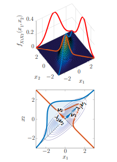
where the terms inside the exponential describe an $n$-dimensional ellipsoid centered at $\boldsymbol{\mu}{\mathbf{X}}$. The directions of the principal axes of this ellipsoid are described by the eigenvector (see \$2.4.2) of the covariance matrix $\boldsymbol{\Sigma}{\mathbf{X}}$, and their lengths by the eigenvalues. Figure $4.3$ presents an example of a covariance matrix decomposed into its eigenvector and eigenvalues. The curves overlaid on the joint PDF describe the marginal PDFs in the eigen space.
For the multivariate Normal joint PDF formulation, the term on the left of the exponential is again the normalization constant, which now includes the determinant of the covariance matrix. As presented in $\S 2.4 .1$, the determinant quantifies how much the covariance matrix $\mathbf{\Sigma}{\mathbf{X}}$ is scaling the space $\mathbf{x}$. Figure $4.4$ presents examples of bivariate Normal PDF and CDF with parameters $\mu{1}=0, \sigma_{1}=2, \mu_{2}=0, \sigma_{2}=1$, and $\rho=0.6$. For the bivariate CDF, notice how evaluating the upper bound for one variable leads to the marginal CDF, represented by the bold red line, for the other variable.
计算机代写|机器学习代写machine learning代考|Properties
A multivariate Normal random variable follow several properties. Here, we insist on six:
- It is completely defined by its mean vector $\boldsymbol{\mu}_{\mathbf{X}}$ and covariance $\operatorname{matrix} \boldsymbol{\Sigma} \mathbf{X}$.
- Its marginal distributions are also Normal, and the PDF of any marginal is given by
$$
x_{i}: X_{i} \sim \mathcal{N}\left(x_{i} ;\left[\boldsymbol{\mu}{\mathbf{X}}\right]{i}\left[\boldsymbol{\Sigma}{\mathbf{X}}\right]{i i}\right)
$$ - The absence of correlation implies statistical independence. Note that this is not generally true for other types of random variables (see $\$ 3.3 .5$ ),
$$
\rho_{i j}=0 \Leftrightarrow X_{i} \Perp X_{j} .
$$ - The central limit theorem (CLT) states that, under some conditions, the asymptotic distribution obtained from the normalized sum of independent identically distributed (iid) random variables (normally distributed or not) is Normal. Given $X_{i}, \forall i \in{1, \cdots, n}$, a set of iid random variables with expected value $\mathbb{E}\left[X_{i}\right]=\mu_{X}$ and finite variance $\sigma_{X}^{2}$, the PDF of $Y=\sum_{i=1}^{n} X_{i}$ approaches $\mathcal{N}\left(n \mu_{X}, n \sigma_{X}^{2}\right)$, for $n \rightarrow \infty$. More formally, the CLT states that
$$
\sqrt{n}\left(\frac{Y}{n}-\mu_{X}\right) \stackrel{d}{\rightarrow} \mathcal{N}\left(0, \sigma_{X}^{2}\right)
$$
where $\stackrel{d}{\rightarrow}$ means converges in distribution. In practice, when obacrving the outcomes of real-life phenomena, it is common to obtain empirical distributions that are similar to the Normal distribution. We can see the parallel where these phenomena are themselves issued from the superposition of several phenomena. This property is key in explaining the widespread usage of the Normal probability distribution. - The output from linear functions of Normal random variables are also Normal. Given $\mathbf{x}: \mathbf{X} \sim \mathcal{N}\left(\mathbf{x} ; \boldsymbol{\mu}{\mathbf{X}}, \mathbf{\Sigma}{\mathbf{X}}\right)$ and a linear function $\mathbf{y}=\mathbf{A x}+\mathbf{b}$, the properties of linear transformations described in \$3.4.1 allow obtaining
$$
\mathbf{Y} \sim \mathcal{N}\left(\mathbf{y} ; \mathbf{A} \mu \mathbf{x}+\mathbf{b}, \mathbf{A} \mathbf{\Sigma}{\mathbf{X}} \mathbf{A}^{\top}\right) $$ Let us consider the simplified case of a linear function $z=x+y$ for two random variables $x: X \sim \mathcal{N}\left(x ; \mu{X}, \sigma_{X}^{2}\right), y: Y \sim$ $\mathcal{N}\left(y ; \mu_{Y}, \sigma_{Y}^{2}\right)$. Their sum is described by $Z \sim \mathcal{N}\left(z ; \mu_{X}+\mu{Y}, \sigma{X}^{2}+\sigma_{Y}^{2}+2 \rho_{X Y} \sigma_{X} \sigma_{Y}\right) .$
机器学习代考
计算机代写|机器学习代写machine learning代考|Univariate Normal
正态随机变量的概率密度函数 (PDF) 在实数上定义X∈R.X∼ñ(X;μ,σ2)由其均值参数化μ和方差σ2, 所以它的 PDF 是
FX(X)=ñ(X;μ,σ2)=12圆周率σ经验(−12(X−μσ)2)
图 4.1 给出了 PDF 和带有参数的累积分布函数 (CDF) 的示例μ=0和σ=1. 最可能的值对应于平均值的模式。改变平均值μ导致分布的翻译。增加标准差σ导致 PDF 色散的成比例增加。正常 CDF 如图 4.1b 所示。它的公式是通过积分得到的,其中积分可以
使用误差函数 erf(-) 进行公式化,
FX(X)=∫−∞X12圆周率σ经验(−12(X′−μσ)2)dX′ =12(1+继承(X−μσ2))
数字4.2说明了构建单变量正态 PDF 所采取的连续步骤。在 PDF 公式的最里面的括号内是一个线性函数X−μσ, 哪个中心X平均而言μ并用标准差对其进行归一化σ. 然后将第一项平方,在其所有域上得到一个正数,除了平均值,它等于零。取第二项的负指数会导致钟形曲线,其中值等于 1(经验(0)=1)平均而言X=μ以及在哪里有拐点μ±σ. 在这一步,曲线与最终的 Normal PDF 成正比。仅缺少归一化常数以确保∫−∞∞F(X)dX=1. 归一化常数是通过对指数项积分得到的,
∫−∞+∞经验(−12(X−μσ)2)dX=2圆周率σ
将指数项除以方程中的归一化常数4.1得到法线 PDF 的最终公式。请注意,对于X=μ,F(μ)≠1因为 PDF 已经标准化,所以它的积分是一。
计算机代写|机器学习代写machine learning代考|Multivariate Normal
两个正态随机变量的联合概率密度函数 (PDF)\left{X_{1}, X_{2}\right}\left{X_{1}, X_{2}\right}是(谁)给的
FX1X2(X1,X2)=12圆周率σ1σ21−ρ2经验(−12(1−ρ2)((X1−μ1σ1)2+(X2−μ2σ2)2−2ρ(X1−μ1σ1)(X2−μ2σ2)))
指数内的括号内有三个项。
前两个类似于单变量情况的二次项。第三个包含一个新参数ρ描述之间的相关系数X1和X2. 这三个一起 术语描述了以 为中心的二维椭圆方程 [μ1μ2]⊤. 多元正态 X∈Rn:X∼ñ(X;μX,ΣX)随机变量X=[X1X2⋯Xn]⊤描述为X∈Rn :
X∼ñ(X:μX,ΣX), 在哪里μX=[μ1μ2⋯μn]⊤是一个向量
包含平均值和ΣX是协方差矩阵,
ΣX=DXRXD=[σ12ρ12σ1σ2⋯ρ1nσ1σn σ22⋯ρ2nσ2σn ⋯⋮ 符号。 σn2]n×n.DX是包含每个随机变量在其主对角线上的标准差的标准差矩阵,并且RX是包含每对随机变量的相关系数的对称(sym.)相关矩阵,
DX=[σ1000 σ200 ⋱0 符号。 σn],RX=[1ρ12⋯ρ1n 1⋯ρ2n ⋯ρn−1n 符号。 1]
请注意,变量与自身呈线性相关,因此相关矩阵的主要对角项为[RX]一世一世=1, ∀一世. 多元法线联合 PDF 描述为
FX(X)=1(2圆周率)n/2(这ΣX)1/2经验(−12(X−μX)⊤ΣX−1(X−μX)),
其中指数内的项描述了一个n维椭球中心在μX. 该椭球的主轴方向由协方差矩阵的特征向量(见$ 2.4.2)描述ΣX,它们的长度由特征值决定。数字4.3给出了一个协方差矩阵的示例,该矩阵分解为其特征向量和特征值。覆盖在联合 PDF 上的曲线描述了特征空间中的边缘 PDF。
对于多元正态联合 PDF 公式,指数左侧的项再次是归一化常数,现在包括协方差矩阵的行列式。如中所述§§2.4.1, 行列式量化了协方差矩阵的多少ΣX正在缩放空间X. 数字4.4提供带参数的双变量正态 PDF 和 CDF 示例μ1=0,σ1=2,μ2=0,σ2=1, 和ρ=0.6. 对于二元 CDF,请注意评估一个变量的上限如何导致另一个变量的边缘 CDF(由粗红线表示)。
计算机代写|机器学习代写machine learning代考|Properties
多元正态随机变量遵循几个属性。在这里,我们坚持六点:
- 它完全由它的平均向量定义μX和协方差矩阵ΣX.
- 它的边缘分布也是正态分布,任何边缘的 PDF 由下式给出
X一世:X一世∼ñ(X一世;[μX]一世[ΣX]一世一世) - 缺乏相关性意味着统计独立性。请注意,这通常不适用于其他类型的随机变量(参见$3.3.5 ),
ρ一世j=0⇔X一世\珀普Xj. - 中心极限定理 (CLT) 指出,在某些条件下,从独立同分布 (iid) 随机变量(正态分布或非正态分布)的归一化总和获得的渐近分布是正态分布。给定X一世,∀一世∈1,⋯,n,一组具有期望值的独立同分布随机变量和[X一世]=μX和有限方差σX2, 的 PDF是=∑一世=1nX一世方法ñ(nμX,nσX2), 为了n→∞. 更正式地说,CLT 指出
n(是n−μX)→dñ(0,σX2)
在哪里→d均值在分布中收敛。在实践中,在观察现实生活现象的结果时,通常会获得类似于正态分布的经验分布。我们可以看到这些现象本身是从几种现象的叠加中产生的平行线。该属性是解释正态概率分布广泛使用的关键。 - 正态随机变量的线性函数的输出也是正态的。给定X:X∼ñ(X;μX,ΣX)和一个线性函数是=一个X+b, $ 3.4.1中描述的线性变换的属性允许获得
是∼ñ(是;一个μX+b,一个ΣX一个⊤)让我们考虑线性函数的简化情况和=X+是对于两个随机变量X:X∼ñ(X;μX,σX2),是:是∼ ñ(是;μ是,σ是2). 它们的总和由 $Z \sim \mathcal{N}\left(z ; \mu_{X}+ \mu {Y}, \sigma{X}^{2}+\sigma_{Y}^{2} 描述+2 \rho_{XY} \sigma_{X} \sigma_{Y}\right) .$

统计代写请认准statistics-lab™. statistics-lab™为您的留学生涯保驾护航。
金融工程代写
金融工程是使用数学技术来解决金融问题。金融工程使用计算机科学、统计学、经济学和应用数学领域的工具和知识来解决当前的金融问题,以及设计新的和创新的金融产品。
非参数统计代写
非参数统计指的是一种统计方法,其中不假设数据来自于由少数参数决定的规定模型;这种模型的例子包括正态分布模型和线性回归模型。
广义线性模型代考
广义线性模型(GLM)归属统计学领域,是一种应用灵活的线性回归模型。该模型允许因变量的偏差分布有除了正态分布之外的其它分布。
术语 广义线性模型(GLM)通常是指给定连续和/或分类预测因素的连续响应变量的常规线性回归模型。它包括多元线性回归,以及方差分析和方差分析(仅含固定效应)。
有限元方法代写
有限元方法(FEM)是一种流行的方法,用于数值解决工程和数学建模中出现的微分方程。典型的问题领域包括结构分析、传热、流体流动、质量运输和电磁势等传统领域。
有限元是一种通用的数值方法,用于解决两个或三个空间变量的偏微分方程(即一些边界值问题)。为了解决一个问题,有限元将一个大系统细分为更小、更简单的部分,称为有限元。这是通过在空间维度上的特定空间离散化来实现的,它是通过构建对象的网格来实现的:用于求解的数值域,它有有限数量的点。边界值问题的有限元方法表述最终导致一个代数方程组。该方法在域上对未知函数进行逼近。[1] 然后将模拟这些有限元的简单方程组合成一个更大的方程系统,以模拟整个问题。然后,有限元通过变化微积分使相关的误差函数最小化来逼近一个解决方案。
tatistics-lab作为专业的留学生服务机构,多年来已为美国、英国、加拿大、澳洲等留学热门地的学生提供专业的学术服务,包括但不限于Essay代写,Assignment代写,Dissertation代写,Report代写,小组作业代写,Proposal代写,Paper代写,Presentation代写,计算机作业代写,论文修改和润色,网课代做,exam代考等等。写作范围涵盖高中,本科,研究生等海外留学全阶段,辐射金融,经济学,会计学,审计学,管理学等全球99%专业科目。写作团队既有专业英语母语作者,也有海外名校硕博留学生,每位写作老师都拥有过硬的语言能力,专业的学科背景和学术写作经验。我们承诺100%原创,100%专业,100%准时,100%满意。
随机分析代写
随机微积分是数学的一个分支,对随机过程进行操作。它允许为随机过程的积分定义一个关于随机过程的一致的积分理论。这个领域是由日本数学家伊藤清在第二次世界大战期间创建并开始的。
时间序列分析代写
随机过程,是依赖于参数的一组随机变量的全体,参数通常是时间。 随机变量是随机现象的数量表现,其时间序列是一组按照时间发生先后顺序进行排列的数据点序列。通常一组时间序列的时间间隔为一恒定值(如1秒,5分钟,12小时,7天,1年),因此时间序列可以作为离散时间数据进行分析处理。研究时间序列数据的意义在于现实中,往往需要研究某个事物其随时间发展变化的规律。这就需要通过研究该事物过去发展的历史记录,以得到其自身发展的规律。
回归分析代写
多元回归分析渐进(Multiple Regression Analysis Asymptotics)属于计量经济学领域,主要是一种数学上的统计分析方法,可以分析复杂情况下各影响因素的数学关系,在自然科学、社会和经济学等多个领域内应用广泛。
MATLAB代写
MATLAB 是一种用于技术计算的高性能语言。它将计算、可视化和编程集成在一个易于使用的环境中,其中问题和解决方案以熟悉的数学符号表示。典型用途包括:数学和计算算法开发建模、仿真和原型制作数据分析、探索和可视化科学和工程图形应用程序开发,包括图形用户界面构建MATLAB 是一个交互式系统,其基本数据元素是一个不需要维度的数组。这使您可以解决许多技术计算问题,尤其是那些具有矩阵和向量公式的问题,而只需用 C 或 Fortran 等标量非交互式语言编写程序所需的时间的一小部分。MATLAB 名称代表矩阵实验室。MATLAB 最初的编写目的是提供对由 LINPACK 和 EISPACK 项目开发的矩阵软件的轻松访问,这两个项目共同代表了矩阵计算软件的最新技术。MATLAB 经过多年的发展,得到了许多用户的投入。在大学环境中,它是数学、工程和科学入门和高级课程的标准教学工具。在工业领域,MATLAB 是高效研究、开发和分析的首选工具。MATLAB 具有一系列称为工具箱的特定于应用程序的解决方案。对于大多数 MATLAB 用户来说非常重要,工具箱允许您学习和应用专业技术。工具箱是 MATLAB 函数(M 文件)的综合集合,可扩展 MATLAB 环境以解决特定类别的问题。可用工具箱的领域包括信号处理、控制系统、神经网络、模糊逻辑、小波、仿真等。