如果你也在 怎样代写利率建模Interest Rate Modeling这个学科遇到相关的难题,请随时右上角联系我们的24/7代写客服。
利率模型是指一种对利率的运动和演变进行建模的数学方法。它是一种基于市场风险的单因素短利率模型。瓦西克利率模型常用于经济学中,以确定利率在未来的移动方向。
statistics-lab™ 为您的留学生涯保驾护航 在代写利率建模Interest Rate Modeling方面已经树立了自己的口碑, 保证靠谱, 高质且原创的统计Statistics代写服务。我们的专家在代写利率建模Interest Rate Modeling代写方面经验极为丰富,各种代写利率建模Interest Rate Modeling相关的作业也就用不着说。
我们提供的利率建模Interest Rate Modeling及其相关学科的代写,服务范围广, 其中包括但不限于:
- Statistical Inference 统计推断
- Statistical Computing 统计计算
- Advanced Probability Theory 高等概率论
- Advanced Mathematical Statistics 高等数理统计学
- (Generalized) Linear Models 广义线性模型
- Statistical Machine Learning 统计机器学习
- Longitudinal Data Analysis 纵向数据分析
- Foundations of Data Science 数据科学基础
金融代写|利率建模代写Interest Rate Modeling代考|Simple Random Walks
Simple random walks are discrete time series, $\left{X_{i}\right}$, defined as
$$
\begin{aligned}
X_{0} &=0, \
X_{n+1} &= \begin{cases}X_{n}-\sqrt{\Delta t}, & p=\frac{1}{2} \
X_{n}+\sqrt{\Delta t}, & 1-p=\frac{1}{2}\end{cases}
\end{aligned}
$$
where $\Delta t>0$ stands for the interval of time for stepping forward. One can verify that $\left{X_{i}\right}$ have the following properties:
- The increment of $X_{n+1}-X_{n}$ is independent of $\left{X_{i}\right}, \forall i \leq n$.
- $E\left[X_{n} \mid X_{m}\right]=X_{m}, m \leq n$.
- $\operatorname{Var}\left[X_{n} \mid X_{m}\right]=(n-m) \Delta t, m \leq n$.
An interesting feature of the simple random walk is the linearity of $X_{i}$ ‘s variance in time: given $X_{0}$, the variance of $X_{i}$ is equal to $i \Delta t$, the time it takes the time series to evolve from $X_{0}$ to $X_{i}$.
Out of the simple Brownian random walk, we can construct a continuous-time process through linear interpolation:
$$
\bar{X}(t)=X_{i}+\frac{t-i \Delta t}{\Delta t}\left(X_{i+1}-X_{i}\right), \quad t \in[i \Delta t,(i+1) \Delta t]
$$
We are interested in the limiting process of $\bar{X}(t)$ as $\Delta t \rightarrow 0$, in the hope that the limit remains a meaningful stochastic process. The next theorem confirms just that.
金融代写|利率建模代写Interest Rate Modeling代考|Brownian Motion
A continuous stochastic process is a collection of real-valued random variables, ${X(t, \omega), 0 \leq t \leq T}$ or $\left{X_{t}(\omega), 0 \leq t \leq T\right}$, that are defined on a probability space $(\Omega, \mathcal{F}, \mathbb{P})$. Here $\Omega$ is the collection of all $\omega$ s, which are so-called sample points, $\mathcal{F}$ the smallest $\sigma$-algebra that contains $\Omega$, and $\mathbb{P}$ a probability measure on $\Omega$. Each random outcome, $\omega \in \Omega$, corresponds to an entire time series
$$
t \rightarrow X_{t}(\omega), \quad t \in T
$$
which is called a path of $X_{t}$. In view of Equation 1.7, we can regard $X_{t}(\omega)$ as a function of two variables, $\omega$ and $t$. For notational simplicity, however, we often suppress the $\omega$ variable when its explicit appearance is not necessary.
In the context of financial modeling, we are particularly interested in the Brownian motion introduced earlier. Its formal definition is given below.
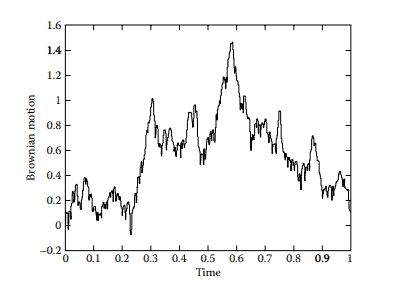
Definition 1.1 A Brownian motion or a Wiener process is a realvalued stochastic process, $W_{t}$ or $W(t), 0 \leq t \leq \infty$, that has the following properties:
- $W(0)=0$.
- $W(t+s)-W(t)$ is independent of ${W(u), 0 \leq u \leq t}$.
- For $t \geq 0$ and $s>0$, the increment $W(t+s)-W(t) \sim N(0, s)$.
- $W(t)$ is continuous almost surely (a.s.).
Here $N(0, s)$ stands for a normal distribution with mean zero and variance s. Note that in some literature, property 4 is not part of the definition, as it can be proved to be implied by the first three properties (Varadhan, $1980 \mathrm{a}$ or Ikeda and Watanabe, 1989). A sample path of $W(t)$ is shown in Figure $1.1$, which is generated with a step size of $\Delta t=2^{-10}$.
Brownian motion plays a major role in continuous time stochastic modeling in physics, engineering and finance. In finance, it has been used to model the random behavior of asset returns. Several major properties of Brownian motion are listed below.
金融代写|利率建模代写Interest Rate Modeling代考|STOCHASTIC INTEGRALS
Stochastic calculus considers the integration and differentiation of general $\mathcal{F}{t}$-adaptive functions. The purpose of developing such a stochastic calculus is to model financial time series (with random dynamics) with either integral or differential equations. According to Lemma 1.1, a Brownian motion, $W(t)$, is nowhere differentiable in the usual sense of differentiation for deterministic functions. To define differentials of stochastic processes in a proper sense, we must first study the notion of stochastic integrals. Stochastic integrals can be defined for functions in the square-integrable space, $H^{2}[0, T]=L^{2}(\Omega \times[0, T], \mathrm{d} \mathbb{P} \times \mathrm{d} t)$, which is defined to be the collection of functions satisfying $$ E\left[\int{0}^{T}|f(t, \omega)|^{2} \mathrm{~d} t\right]<\infty
$$
Note that, without indicated otherwise, $E[\cdot]$ means $E^{\mathbb{P}}[\cdot]$, the unconditional expectation under $\mathbb{P}$. The definition consists of a three-step procedure. First, we make the definition for elementary or piecewise constant functions in an intuitive way. Second, we define the integrals of a bounded continuous function as a limit of integrals of elementary functions. Finally, we define the integral of a general square-integrable function as a limit of integrals of bounded continuous functions. The key in this three-step procedure is of course to ensure the convergence of the limits in $L^{2}(\Omega, \mathcal{F}, \mathbb{P})$, the Hilbert space of random variables satisfying
$$
E\left[X^{2}(\omega)\right]<\infty
$$
This definition approach is taken by Oksendal (1992). Alternative treatments of course also exist; see, for example, Mikosch (1998).
利率建模代考
金融代写|利率建模代写Interest Rate Modeling代考|Simple Random Walks
简单的随机游走是离散的时间序列, left{X_{i}}right }, 定义为
$$
X_{0}=0, X_{n+1} \quad=\left{X_{n}-\sqrt{\Delta t}, \quad p=\frac{1}{2} X_{n}+\sqrt{\Delta t}, \quad 1-p=\frac{1}{2}\right.
$$
在哪里 $\Delta t>0$ 代表前进的时间间隔。可以验证 lleft{X_{i}}right} $}$ 具有以下属性:
- 的增量 $X_{n+1}-X_{n}$ 独立于⿴left $\left{X_{-}{i} \backslash\right.$ Iight}, Iforall i leq n.
- $E\left[X_{n} \mid X_{m}\right]=X_{m}, m \leq n$.
- $\operatorname{Var}\left[X_{n} \mid X_{m}\right]=(n-m) \Delta t, m \leq n$.
简单随机游走的一个有趣特征是 $X_{i}$ 的时间变化: 给定 $X_{0}$, 的方差 $X_{i}$ 等于 $i \Delta t$, 时间序列从 $X_{0}$ 至 $X_{i}$.
从简单的布朗随机游走中,我们可以通过线性揷值构造一个连续时间的过程:
$$
\bar{X}(t)=X_{i}+\frac{t-i \Delta t}{\Delta t}\left(X_{i+1}-X_{i}\right), \quad t \in[i \Delta t,(i+1) \Delta t]
$$
我们对限制过程感兴趣 $\bar{X}(t)$ 作为 $\Delta t \rightarrow 0$ ,希望极限仍然是一个有意义的随机过程。下一个定理证实了这一点。
金融代写|利率建模代写Interest Rate Modeling代考|Brownian Motion
连续随机过程是实值随机变量的集合, $X(t, \omega), 0 \leq t \leq T$ 或者 Ueft $\left{X_{-} \mathrm{~ { t } (}\right.$ 间上定义 $(\Omega, \mathcal{F}, \mathbb{P})$. 这里 $\Omega$ 是所有的集合 $\omega \mathrm{s}$ ,即所谓的样本点, $\mathcal{F}$ 最小的 $\sigma$-代数包含 $\Omega$ ,和 $\mathbb{P}$ 概率测度 $\Omega$. 每个随 机结果, $\omega \in \Omega$ ,对应于整个时间序列
$$
t \rightarrow X_{t}(\omega), \quad t \in T
$$
这被称为路径 $X_{t}$. 鉴于公式 1.7,我们可以认为 $X_{t}(\omega)$ 作为两个变量的函数, $\omega$ 和 $t$. 然而,为了符号的简单性,我 们经常抑制 $\omega$ 不需要显式外观时的变量。
在金融建模的背景下,我们对前面介绍的布朗运动特别感兴趣。其正式定义如下。
定义 $1.1$ 布朗运动或维纳过程是实值随机过程, $W_{t}$ 或者 $W(t), 0 \leq t \leq \infty$ ,具有以下性质:
- $W(0)=0$.
- $W(t+s)-W(t)$ 独立于 $W(u), 0 \leq u \leq t$.
- 为了 $t \geq 0$ 和 $s>0$, 增量 $W(t+s)-W(t) \sim N(0, s)$.
- $W(t)$ 几平肯定是连续的 (as)。
这里 $N(0, s)$ 代表均值为零且方差为 $\mathrm{s}$ 的正态分布。请注意,在某些文献中,属性 4 不是定义的一部分,因 为可以证明前三个属性暗示了它 (Varadhan,1980a或池田和渡边,1989) 。一个示例路径 $W(t)$ 如图1.1 ,它的生成步长为 $\Delta t=2^{-10}$.
布朗运动在物理学、工程和金融领域的连续时间随机建模中发挥着重要作用。在金融领域,它已被用于模拟资产回 报的随机行为。下面列出了布朗运动的几个主要性质。
金融代写|利率建模代写Interest Rate Modeling代考|STOCHASTIC INTEGRALS
随机微积分考虑一般的积分和微分 $\mathcal{F} t$ – 自适应功能。开发这种随机微积分的目的是用积分或微分方程对金融时间序 列 (具有随机动力学) 进行建模。根据引理 1.1,布朗运动, $W(t)$ ,在确定性函数的通常微分意义上是不可微的。 为了正确定义随机过程的微分,我们必须首先研究随机积分的概念。可以为平方可积空间中的函数定义随机积分, $H^{2}[0, T]=L^{2}(\Omega \times[0, T], \mathrm{d} \mathbb{P} \times \mathrm{d} t)$ ,它被定义为满足的函数的集合
$$
E\left[\int 0^{T}|f(t, \omega)|^{2} \mathrm{~d} t\right]<\infty
$$
请注意,在没有另外说明的情况下, $E[\cdot]$ 方法 $E^{\mathbb{P}}[\cdot]$, 下的无条件期望 $\mathbb{P}$. 该定义包括一个三步程序。首先,我们以 直观的方式定义基本或分段常数函数。其次,我们将有界连续函数的积分定义为初等函数积分的极限。最后,我们 将一般平方可积函数的积分定义为有界连续函数积分的极限。这个三步程序的关键当然是确保在 $L^{2}(\Omega, \mathcal{F}, \mathbb{P})$ ,随 机变量的希尔伯特空间满足
$$
E\left[X^{2}(\omega)\right]<\infty
$$
Oksendal (1992) 采用了这种定义方法。当然也存在替代疗法;例如,参见 Mikosch (1998)。

统计代写请认准statistics-lab™. statistics-lab™为您的留学生涯保驾护航。
金融工程代写
金融工程是使用数学技术来解决金融问题。金融工程使用计算机科学、统计学、经济学和应用数学领域的工具和知识来解决当前的金融问题,以及设计新的和创新的金融产品。
非参数统计代写
非参数统计指的是一种统计方法,其中不假设数据来自于由少数参数决定的规定模型;这种模型的例子包括正态分布模型和线性回归模型。
广义线性模型代考
广义线性模型(GLM)归属统计学领域,是一种应用灵活的线性回归模型。该模型允许因变量的偏差分布有除了正态分布之外的其它分布。
术语 广义线性模型(GLM)通常是指给定连续和/或分类预测因素的连续响应变量的常规线性回归模型。它包括多元线性回归,以及方差分析和方差分析(仅含固定效应)。
有限元方法代写
有限元方法(FEM)是一种流行的方法,用于数值解决工程和数学建模中出现的微分方程。典型的问题领域包括结构分析、传热、流体流动、质量运输和电磁势等传统领域。
有限元是一种通用的数值方法,用于解决两个或三个空间变量的偏微分方程(即一些边界值问题)。为了解决一个问题,有限元将一个大系统细分为更小、更简单的部分,称为有限元。这是通过在空间维度上的特定空间离散化来实现的,它是通过构建对象的网格来实现的:用于求解的数值域,它有有限数量的点。边界值问题的有限元方法表述最终导致一个代数方程组。该方法在域上对未知函数进行逼近。[1] 然后将模拟这些有限元的简单方程组合成一个更大的方程系统,以模拟整个问题。然后,有限元通过变化微积分使相关的误差函数最小化来逼近一个解决方案。
tatistics-lab作为专业的留学生服务机构,多年来已为美国、英国、加拿大、澳洲等留学热门地的学生提供专业的学术服务,包括但不限于Essay代写,Assignment代写,Dissertation代写,Report代写,小组作业代写,Proposal代写,Paper代写,Presentation代写,计算机作业代写,论文修改和润色,网课代做,exam代考等等。写作范围涵盖高中,本科,研究生等海外留学全阶段,辐射金融,经济学,会计学,审计学,管理学等全球99%专业科目。写作团队既有专业英语母语作者,也有海外名校硕博留学生,每位写作老师都拥有过硬的语言能力,专业的学科背景和学术写作经验。我们承诺100%原创,100%专业,100%准时,100%满意。
随机分析代写
随机微积分是数学的一个分支,对随机过程进行操作。它允许为随机过程的积分定义一个关于随机过程的一致的积分理论。这个领域是由日本数学家伊藤清在第二次世界大战期间创建并开始的。
时间序列分析代写
随机过程,是依赖于参数的一组随机变量的全体,参数通常是时间。 随机变量是随机现象的数量表现,其时间序列是一组按照时间发生先后顺序进行排列的数据点序列。通常一组时间序列的时间间隔为一恒定值(如1秒,5分钟,12小时,7天,1年),因此时间序列可以作为离散时间数据进行分析处理。研究时间序列数据的意义在于现实中,往往需要研究某个事物其随时间发展变化的规律。这就需要通过研究该事物过去发展的历史记录,以得到其自身发展的规律。
回归分析代写
多元回归分析渐进(Multiple Regression Analysis Asymptotics)属于计量经济学领域,主要是一种数学上的统计分析方法,可以分析复杂情况下各影响因素的数学关系,在自然科学、社会和经济学等多个领域内应用广泛。
MATLAB代写
MATLAB 是一种用于技术计算的高性能语言。它将计算、可视化和编程集成在一个易于使用的环境中,其中问题和解决方案以熟悉的数学符号表示。典型用途包括:数学和计算算法开发建模、仿真和原型制作数据分析、探索和可视化科学和工程图形应用程序开发,包括图形用户界面构建MATLAB 是一个交互式系统,其基本数据元素是一个不需要维度的数组。这使您可以解决许多技术计算问题,尤其是那些具有矩阵和向量公式的问题,而只需用 C 或 Fortran 等标量非交互式语言编写程序所需的时间的一小部分。MATLAB 名称代表矩阵实验室。MATLAB 最初的编写目的是提供对由 LINPACK 和 EISPACK 项目开发的矩阵软件的轻松访问,这两个项目共同代表了矩阵计算软件的最新技术。MATLAB 经过多年的发展,得到了许多用户的投入。在大学环境中,它是数学、工程和科学入门和高级课程的标准教学工具。在工业领域,MATLAB 是高效研究、开发和分析的首选工具。MATLAB 具有一系列称为工具箱的特定于应用程序的解决方案。对于大多数 MATLAB 用户来说非常重要,工具箱允许您学习和应用专业技术。工具箱是 MATLAB 函数(M 文件)的综合集合,可扩展 MATLAB 环境以解决特定类别的问题。可用工具箱的领域包括信号处理、控制系统、神经网络、模糊逻辑、小波、仿真等。