如果你也在 怎样代写利率建模Interest Rate Modeling这个学科遇到相关的难题,请随时右上角联系我们的24/7代写客服。
利率模型是指一种对利率的运动和演变进行建模的数学方法。它是一种基于市场风险的单因素短利率模型。瓦西克利率模型常用于经济学中,以确定利率在未来的移动方向。
statistics-lab™ 为您的留学生涯保驾护航 在代写利率建模Interest Rate Modeling方面已经树立了自己的口碑, 保证靠谱, 高质且原创的统计Statistics代写服务。我们的专家在代写利率建模Interest Rate Modeling代写方面经验极为丰富,各种代写利率建模Interest Rate Modeling相关的作业也就用不着说。
我们提供的利率建模Interest Rate Modeling及其相关学科的代写,服务范围广, 其中包括但不限于:
- Statistical Inference 统计推断
- Statistical Computing 统计计算
- Advanced Probability Theory 高等概率论
- Advanced Mathematical Statistics 高等数理统计学
- (Generalized) Linear Models 广义线性模型
- Statistical Machine Learning 统计机器学习
- Longitudinal Data Analysis 纵向数据分析
- Foundations of Data Science 数据科学基础
金融代写|利率建模代写Interest Rate Modeling代考|Nested Simulation
There are many exotic options whose price depends on the path of an underlying asset. If a structured product involves an exotic derivative, then the price of the product is also path-dependent. Since the pricing of complex products is not trivial, recombining trees and Monte Carlo simulation are employed for pricing.
When a portfolio contains exotic products such as those described above, it is difficult to price them for a future date, which is necessary for measuring VaR. Nested simulation is a computing technique for measuring VaR of a derivatives portfolio, which we briefly introduce below.
Let $T$ be a holding period for measuring VaR. We denote by $x_{t}$ the value of the risk factor at time $t$, and by $p_{T}$ the price of a derivative asset at $T$. As illustrated in Fig. $1.8$, the distribution of the risk factor $x_{T}$ at $T$ is simulated by a Monte Carlo method in the outer step. Then, we consider $x_{T}$ to represent a scenario in which VaR is to be measured. At each scenario $x_{T}$, the derivative is priced as $p_{T} \mid x_{T}$ by another Monte Carlo simulation starting at time $T$. This is the inner step. Once we obtain the distribution of $p_{T} \mid x_{T}$, we can compute the VaR in the manner described in Section 1.6.3 of this chapter.
A problem intrinsic to nested simulation is that the number of simulation becomes enormous. There are many studies on algorithms for accelerating nested simulation. As examples, see Devineau and Loisel (2009) and Gordy and Juneja (2010), among others.
金融代写|利率建模代写Interest Rate Modeling代考|Validity of VaR
VaR is widely used as a risk measure in regulatory guidelines in the banking sectors. However it is known that VaR at a particular confidence level does not tell us the loss beyond that level, although the validity of VaR has been studied mathematically and financially in many papers. In this section, we make some brief remarks about the properties of $\mathrm{VaR}$ as a downside risk measure and define expected shortfall as a coherent risk measure. We address these issues basically according to the Bank for International Settlement (BIS, 2004b) for tail risk and according to Artzner et al. (1999) for coherent risk measures.
For this purpose, we denote by $X$ the value of a portfolio at time $T$, and by $\rho$ a risk measure for $X$. Then, $\rho(X)$ represents the size of the risk of $X$ measured by $\rho$. Naturally, the portfolio is allowed to sell some options, which creates the possibility that $X$ will take a negative value. To avoid confusion, we note that a large positive $\rho(X)$ represents a larger risk than a small positive or negative $\rho(X)$. We remark that up to the previous section, risk measures have been defined in terms of the profit-loss measures of a portfolio, such as sensitivity, convexity, and VaR. In this section, we work with a risk measure for $X$ that does not represent profit or loss. In this context, we define a VaR of $V_{\alpha}$ at confidence level $1-\alpha$ over a holding period $T$ as
$$
V_{\alpha}(X)=-\inf {x \mid \mathbf{P}(X \leq x)>\alpha}
$$
Tail risk
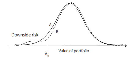
To explain the tail risk, we consider two portfolios, whose prices at time $T$ are denoted by $A$ for one portfolio and $B$ for the other. We use $A$ and $B$ as the names of these portfolios. We assume that $A$ and $B$ have the same VaR at confidence level $1-\alpha$, so that $V_{\alpha}(A)=V_{\alpha}(B)$. In Fig. $1.9$, the solid line shows
the distribution of future value of $A$, and the dashed line shows that of $B$. We see that the downside risk of portfolio $B$ is larger than that of $A$. This shows that $V a R_{\alpha}$ does not capture the difference in downside risk between portfolios, as exemplified by $A$ and $B$; this risk is noted in BIS (2004b) as tail risk.
Under VaR regulations, risk managers will choose portfolio $B$ in preference to A because there is a larger opportunity for profit in B. Thus, VaR might mislead risk managers who optimally control their portfolios. For further argument along these lines, see Basak and Shapiro (2001) and Yamai and Yoshiba $(2002)$, among others.
金融代写|利率建模代写Interest Rate Modeling代考|Probability Space
Probability space
We denote by $\Omega$ a set of all possible outcomes, called the sample space, and an element $w \in \Omega$, called a sample. The family $\mathcal{F}$ is a collection of subsets of $\Omega$ and is assumed to be a $\sigma$-algebra. A stochastic event $A$ is represented as an element in $\mathcal{F}$.
The function $\mathbf{P}$ is a probability function defined on $\mathcal{F}$ such that $\mathbf{P}(\Omega)=1$ and $\mathbf{P}(\phi)=0 ;$ this is also called a probability measure. For $A \in \mathcal{F}, \mathbf{P}(\mathbf{A})$ indicates probability of event $A$ occurring. From these, we characterize a probability space by a triplet $(\Omega, \mathcal{F}, \mathbf{P})$.
Example 2.1: Sample space
In financial engineering, a sample $w \in \Omega$ is regarded as a history of up and down moves of a stock price observed in a fixed period. This makes $\Omega$ the set of up and down sequences of the stock price. If a period consists of two days $\left{t_{1}, t_{2}\right}$, then $\Omega$ will contain four samples and be given by
$$
\Omega={u u, u d, d u, d d}
$$
where we represent by $u$ and $d$ the up and down movements, respectively, of the stock price. Accordingly, $\mathcal{F}$ consists of all subsets of $\Omega$,
$$
\mathcal{F}={\phi, \Omega, u u, u d, d u, d d,{u u, u d},{u u, d d,}, \cdots}
$$
which means that $\mathcal{F}$ has $16\left(=2^{4}\right)$ events.
Real-world measure
In financial market analysis, the probability measure derived from observation of market prices is called the market measure, with many synonyms, such as historical measure, physical measure, actual measure, and real-world measure. We regard historical data as being observed under the real-world measure.
Recall the previous example. If our observation estimates that the probability of an up move is constant at $0.5$ and the down-move probability is $0.5$, then we have
$$
\mathbf{P}(u u)=\mathbf{P}(u d)=\mathbf{P}(d u)=\mathbf{P}(d d)=0.25
$$
Accordingly, for an arbitrary event $A \in \mathcal{F}$, it is possible to give $\mathbf{P}(A)$. This probability measure $\mathbf{P}$ is an example of the real-world measure.
利率建模代考
金融代写|利率建模代写Interest Rate Modeling代考|Nested Simulation
有许多奇异期权的价格取决于标的资产的路径。如果结构性产品涉及奇异衍生品,那么产品的价格也是路径相关的。由于复杂产品的定价并非易事,因此采用重组树和蒙特卡罗模拟进行定价。
当投资组合包含如上所述的奇特产品时,很难为将来的日期定价,这对于衡量 VaR 是必要的。嵌套模拟是一种用于衡量衍生品投资组合 VaR 的计算技术,我们将在下面简要介绍。
让吨是衡量 VaR 的持有期。我们表示X吨风险因素在时间的价值吨,并由p吨衍生资产的价格吨. 如图所示。1.8, 风险因素的分布X吨在吨在外部步骤中通过蒙特卡洛方法进行模拟。那么,我们考虑X吨表示要测量 VaR 的情景。在每个场景X吨,衍生品定价为p吨∣X吨由另一个从时间开始的蒙特卡洛模拟吨. 这是内在的步骤。一旦我们得到分布p吨∣X吨,我们可以按照本章 1.6.3 节中描述的方式计算 VaR。
嵌套模拟的一个内在问题是模拟的数量变得巨大。关于加速嵌套仿真的算法有很多研究。例如,参见 Devineau 和 Loisel (2009) 以及 Gordy 和 Juneja (2010) 等。
金融代写|利率建模代写Interest Rate Modeling代考|Validity of VaR
VaR 被广泛用作银行业监管指南中的风险度量。然而,众所周知,特定置信水平的 VaR 并不能告诉我们超出该水平的损失,尽管在许多论文中已经对 VaR 的有效性进行了数学和财务研究。在本节中,我们对属性的一些简要说明在一个R作为下行风险衡量标准,并将预期短缺定义为连贯的风险衡量标准。我们基本上根据国际清算银行 (BIS, 2004b) 的尾部风险和 Artzner 等人的方法来解决这些问题。(1999) 用于连贯的风险措施。
为此,我们记为X投资组合当时的价值吨,并由ρ风险度量X. 然后,ρ(X)代表风险的大小X通过测量ρ. 自然地,投资组合被允许出售一些期权,这创造了以下可能性:X将取负值。为避免混淆,我们注意到一个大的正ρ(X)代表比小的正面或负面更大的风险ρ(X). 我们注意到,直到上一节,风险度量都是根据投资组合的损益度量来定义的,例如敏感性、凸性和 VaR。在本节中,我们使用风险度量X不代表利润或损失。在这种情况下,我们定义 VaR 为在一个在置信水平1−一个持有期吨作为
在一个(X)=−信息X∣磷(X≤X)>一个
尾部风险
为了解释尾部风险,我们考虑两个投资组合,它们的价格吨表示为一个对于一个投资组合和乙对于另一个。我们用一个和乙作为这些投资组合的名称。我们假设一个和乙在置信水平上具有相同的 VaR1−一个, 以便在一个(一个)=在一个(乙). 在图。1.9,实线表示
未来价值的分布一个, 虚线表示乙. 我们看到投资组合的下行风险乙大于一个. 这表明在一个R一个没有捕捉投资组合之间下行风险的差异,例如一个和乙; 这种风险在 BIS (2004b) 中被称为尾部风险。
在 VaR 规定下,风险管理者将选择投资组合乙优先于 A,因为 B 有更大的获利机会。因此,VaR 可能会误导最佳控制其投资组合的风险经理。有关这些方面的进一步论点,请参见 Basak 和 Shapiro (2001) 以及 Yamai 和 Yoshiba(2002),等等。
金融代写|利率建模代写Interest Rate Modeling代考|Probability Space
概率空间
我们表示为Ω一组所有可能的结果,称为样本空间和一个元素在∈Ω,称为样本。家庭F是子集的集合Ω并假定为σ-代数。随机事件一个表示为一个元素F.
功能磷是一个概率函数定义在F这样磷(Ω)=1和磷(φ)=0;这也称为概率测度。为了一个∈F,磷(一个)表示事件的概率一个发生。根据这些,我们用三元组来表征概率空间(Ω,F,磷).
例 2.1:样本空间
在金融工程中,样本在∈Ω被认为是在固定时期内观察到的股票价格上下波动的历史。这使得Ω股票价格的上涨和下跌序列的集合。如果一个时期由两天组成\left{t_{1}, t_{2}\right}\left{t_{1}, t_{2}\right}, 然后Ω将包含四个样本并由下式给出
Ω=在在,在d,d在,dd
我们代表的地方在和d分别是股价的上涨和下跌。因此,F由所有子集组成Ω,
F=φ,Ω,在在,在d,d在,dd,在在,在d,在在,dd,,⋯
意思就是F有16(=24)事件。
真实世界测度
在金融市场分析中,通过观察市场价格得出的概率测度称为市场测度,有许多同义词,如历史测度、物理测度、实际测度和真实世界测度。我们认为历史数据是在现实世界的衡量标准下观察到的。
回想一下前面的例子。如果我们的观察估计上涨的概率是恒定的0.5向下移动的概率是0.5,那么我们有
磷(在在)=磷(在d)=磷(d在)=磷(dd)=0.25
因此,对于任意事件一个∈F, 可以给磷(一个). 这种概率测度磷是真实世界测量的一个例子。

统计代写请认准statistics-lab™. statistics-lab™为您的留学生涯保驾护航。
金融工程代写
金融工程是使用数学技术来解决金融问题。金融工程使用计算机科学、统计学、经济学和应用数学领域的工具和知识来解决当前的金融问题,以及设计新的和创新的金融产品。
非参数统计代写
非参数统计指的是一种统计方法,其中不假设数据来自于由少数参数决定的规定模型;这种模型的例子包括正态分布模型和线性回归模型。
广义线性模型代考
广义线性模型(GLM)归属统计学领域,是一种应用灵活的线性回归模型。该模型允许因变量的偏差分布有除了正态分布之外的其它分布。
术语 广义线性模型(GLM)通常是指给定连续和/或分类预测因素的连续响应变量的常规线性回归模型。它包括多元线性回归,以及方差分析和方差分析(仅含固定效应)。
有限元方法代写
有限元方法(FEM)是一种流行的方法,用于数值解决工程和数学建模中出现的微分方程。典型的问题领域包括结构分析、传热、流体流动、质量运输和电磁势等传统领域。
有限元是一种通用的数值方法,用于解决两个或三个空间变量的偏微分方程(即一些边界值问题)。为了解决一个问题,有限元将一个大系统细分为更小、更简单的部分,称为有限元。这是通过在空间维度上的特定空间离散化来实现的,它是通过构建对象的网格来实现的:用于求解的数值域,它有有限数量的点。边界值问题的有限元方法表述最终导致一个代数方程组。该方法在域上对未知函数进行逼近。[1] 然后将模拟这些有限元的简单方程组合成一个更大的方程系统,以模拟整个问题。然后,有限元通过变化微积分使相关的误差函数最小化来逼近一个解决方案。
tatistics-lab作为专业的留学生服务机构,多年来已为美国、英国、加拿大、澳洲等留学热门地的学生提供专业的学术服务,包括但不限于Essay代写,Assignment代写,Dissertation代写,Report代写,小组作业代写,Proposal代写,Paper代写,Presentation代写,计算机作业代写,论文修改和润色,网课代做,exam代考等等。写作范围涵盖高中,本科,研究生等海外留学全阶段,辐射金融,经济学,会计学,审计学,管理学等全球99%专业科目。写作团队既有专业英语母语作者,也有海外名校硕博留学生,每位写作老师都拥有过硬的语言能力,专业的学科背景和学术写作经验。我们承诺100%原创,100%专业,100%准时,100%满意。
随机分析代写
随机微积分是数学的一个分支,对随机过程进行操作。它允许为随机过程的积分定义一个关于随机过程的一致的积分理论。这个领域是由日本数学家伊藤清在第二次世界大战期间创建并开始的。
时间序列分析代写
随机过程,是依赖于参数的一组随机变量的全体,参数通常是时间。 随机变量是随机现象的数量表现,其时间序列是一组按照时间发生先后顺序进行排列的数据点序列。通常一组时间序列的时间间隔为一恒定值(如1秒,5分钟,12小时,7天,1年),因此时间序列可以作为离散时间数据进行分析处理。研究时间序列数据的意义在于现实中,往往需要研究某个事物其随时间发展变化的规律。这就需要通过研究该事物过去发展的历史记录,以得到其自身发展的规律。
回归分析代写
多元回归分析渐进(Multiple Regression Analysis Asymptotics)属于计量经济学领域,主要是一种数学上的统计分析方法,可以分析复杂情况下各影响因素的数学关系,在自然科学、社会和经济学等多个领域内应用广泛。
MATLAB代写
MATLAB 是一种用于技术计算的高性能语言。它将计算、可视化和编程集成在一个易于使用的环境中,其中问题和解决方案以熟悉的数学符号表示。典型用途包括:数学和计算算法开发建模、仿真和原型制作数据分析、探索和可视化科学和工程图形应用程序开发,包括图形用户界面构建MATLAB 是一个交互式系统,其基本数据元素是一个不需要维度的数组。这使您可以解决许多技术计算问题,尤其是那些具有矩阵和向量公式的问题,而只需用 C 或 Fortran 等标量非交互式语言编写程序所需的时间的一小部分。MATLAB 名称代表矩阵实验室。MATLAB 最初的编写目的是提供对由 LINPACK 和 EISPACK 项目开发的矩阵软件的轻松访问,这两个项目共同代表了矩阵计算软件的最新技术。MATLAB 经过多年的发展,得到了许多用户的投入。在大学环境中,它是数学、工程和科学入门和高级课程的标准教学工具。在工业领域,MATLAB 是高效研究、开发和分析的首选工具。MATLAB 具有一系列称为工具箱的特定于应用程序的解决方案。对于大多数 MATLAB 用户来说非常重要,工具箱允许您学习和应用专业技术。工具箱是 MATLAB 函数(M 文件)的综合集合,可扩展 MATLAB 环境以解决特定类别的问题。可用工具箱的领域包括信号处理、控制系统、神经网络、模糊逻辑、小波、仿真等。