如果你也在 怎样代写金融数学Financial Mathematics这个学科遇到相关的难题,请随时右上角联系我们的24/7代写客服。
金融数学是将数学方法应用于金融问题。(有时使用的同等名称是定量金融、金融工程、数学金融和计算金融)。它借鉴了概率、统计、随机过程和经济理论的工具。传统上,投资银行、商业银行、对冲基金、保险公司、公司财务部和监管机构将金融数学的方法应用于诸如衍生证券估值、投资组合结构、风险管理和情景模拟等问题。依赖商品的行业(如能源、制造业)也使用金融数学。 定量分析为金融市场和投资过程带来了效率和严谨性,在监管方面也变得越来越重要。
statistics-lab™ 为您的留学生涯保驾护航 在代写金融数学Financial Mathematics方面已经树立了自己的口碑, 保证靠谱, 高质且原创的统计Statistics代写服务。我们的专家在代写金融数学Financial Mathematics代写方面经验极为丰富,各种代写金融数学Financial Mathematics相关的作业也就用不着说。
我们提供的金融数学Financial Mathematics及其相关学科的代写,服务范围广, 其中包括但不限于:
- Statistical Inference 统计推断
- Statistical Computing 统计计算
- Advanced Probability Theory 高等概率论
- Advanced Mathematical Statistics 高等数理统计学
- (Generalized) Linear Models 广义线性模型
- Statistical Machine Learning 统计机器学习
- Longitudinal Data Analysis 纵向数据分析
- Foundations of Data Science 数据科学基础
金融代写|金融数学代写Financial Mathematics代考|The Cox, Ross and Rubinstein model
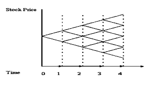
We will now illustrate the different concepts introduced above using a specific case of financial market. This is a discretized version of the Black and Scholes model.
The market is considered to be made up of a risk-free asset $S_{n}^{0}=(1+r)^{n}$ and a single risky asset $S^{1}$ with the dynamic
$$
S_{0}^{1}=1, \quad S_{n+1}^{1}=S_{n}^{1} T_{n+1}, n \geq 0,
$$
where $\left(T_{n}\right){1 \leq n \leq N}$ is a sequence of random variable taking only two values $1+d$ and $1+u$ with $-1{0}={\emptyset, \Omega}, \mathcal{F}{n}=\sigma\left(T{1}, \ldots, T_{n}\right), 1 \leq n \leq N .
$$
In particular, $\mathcal{F}{N}=\sigma\left(T{1}, \ldots, T_{N}\right)=\mathcal{P}(\Omega)$ is the set of subsets of $\Omega$.
We will now characterize viable markets in this model. In order to do this, we start by studying risk-neutral probabilities.
PROPOSITION 5.2.-The discounted prices $\left(\widetilde{S}{n}^{1}\right){0 \leq n \leq N}$ are a martingale under a probability $\mathbb{P}^{}$ if and only if, for any $0 \leq n \leq N-1$, we have $$ \mathbb{E}^{}\left[T_{n+1} \mid \mathcal{F}{n}\right]=1+r, $$ with $\mathbb{E}^{}$ denoting the expectation for the probability $\mathbb{P}^{}$.
PROOF.- Let us proceed through double implication.
Let us assume that the realized price is a martingale. For any $0 \leq n \leq N-1$, we then have
$$
\begin{aligned}
& \mathbb{E}^{}\left[\widetilde{S}{n+1}^{1} \mid \mathcal{F}{n}\right]=\widetilde{S}{n}^{1} \
\Longrightarrow & \mathbb{E}^{}\left[\frac{S_{n+1}^{1}}{(1+r)^{n+1}} \mid \mathcal{F}{n}\right]=\frac{S{n}^{1}}{(1+r)^{n}} \
\Longrightarrow & \mathbb{E}^{*}\left[S_{n}^{1} T_{n+1} \mid \mathcal{F}{n}\right]=S{n}^{1}(1+r)
\end{aligned}
$$
$$
\begin{aligned}
&\Longrightarrow S_{n}^{1} \mathbb{E}^{}\left[T_{n+1} \mid \mathcal{F}{n}\right]=S{n}^{1}(1+r) \
&\Longrightarrow \mathbb{E}^{}\left[T_{n+1} \mid \mathcal{F}{n}\right]=(1+r) \end{aligned} $$ since $S{n}^{1}$ is the $\mathcal{F}{n}$-measurable. Conversely, if for any $0 \leq n \leq N-1$, we have $\mathbb{E}^{}\left[T{n+1} \mid \mathcal{F}{n}\right]=1+r$; therefore $$ \begin{aligned} & \mathbb{E}^{}\left[T{n+1} \mid \mathcal{F}{n}\right]=(1+r) \ \Longrightarrow & S{n}^{1} \mathbb{E}^{}\left[T_{n+1} \mid \mathcal{F}{n}\right]=S{n}^{1}(1+r) \
\Longrightarrow & \mathbb{E}^{}\left[\frac{S_{n+1}^{1}}{(1+r)^{n+1}} \mid \mathcal{F}{n}\right]=\frac{S{n}^{1}}{(1+r)^{n}} \
\Longrightarrow & \mathbb{E}^{*}\left[\widetilde{S}{n+1}^{1} \mid \mathcal{F}{n}\right]=\widetilde{S}{n}^{1} \end{aligned} $$ therefore $\left(\widetilde{S}{n}^{1}\right)$ is indeed a martingale, as the measurability and integrability conditions are satisfied.
金融代写|金融数学代写Financial Mathematics代考|Portfolio optimization
We now study a portfolio optimization problem in the Cox, Ross and Rubinstein model.
Let $V_{0}$ be the wealth of an investor at the time 0 . The investor can invest their money either in a risky asset or in a risk-free asset, following an admissible strategy. We use $\phi_{n}^{0}$ and $\phi_{n}^{1}$ to denote the number of shares in the risk-free asset and the number of shares in the risky asset, respectively, held between the time $n-1$ and $n$. Let $\pi_{n}$ be the proportion of the wealth invested in the risky asset between the instants $n-1$ and $n$, that is,
$$
\pi_{n}=\frac{\phi_{n}^{1} S_{n-1}^{1}}{V_{n-1}}
$$
1) Express $\phi_{n}^{0}$ and $\phi_{n}^{1}$ as the functions of $\pi_{n}, S_{n-1}^{0}, S_{n-1}^{1}$ and $V_{n-1}$ for any $n$.
2) Derive from this that for any $n$, the wealth at the time $n$, after the evolution of the prices and before the redistribution of the portfolio has the value:
$$
V_{n}=\left(\pi_{n} T_{n}+\left(1-\pi_{n}\right)(1+r)\right) V_{n-1}
$$
3) On the same graph and for the same random sampled trajectory, represent the evolution of the risk-free asset and the evolution of the wealth for the following two strategies:
a) The proportion of the wealth invested in the risky asset is fixed over time, at $1 / 4$.
b) The proportion of the wealth invested in the risky asset only takes the values 0 and 1 . It takes the value 1 when the price of a risky asset strictly exceeds that of the risk-free asset, and takes the value 0 when the risky asset is small than or equal to the risk-free asset, while remaining predictable.
We will take the following parameters: initial wealth $V_{0}=1$, the risky asset evolves as per the Cox, Ross and Rubinstein model with parameters $d=-2 \%$, $u=10 \%$ and $q=0.52$, interest rate $r=4 \%$ and duration of investment: $N=100$ periods.
Now consider that the investor’s utility function is logarithmic and we wish to find the strategy $\pi^{}=\left(\pi_{n}^{}\right){1 \leq n \leq N}$ which maximizes the expectation of the utility of the wealth at maturity $N$ : $$ \sup {\pi \text { admissible }} \mathbb{E}\left[\log V_{N}(\pi)\right]
$$
We will accept that the optimal strategy is constant over time and maximize the expression
$$
q \log \left(\pi^{}(u-r)+1+r\right)+(1-q) \log \left(\pi^{}(d-r)+1+r\right)
$$
We wish to compare the performances of strategies 1 and 2 , given above, and that of the optimal strategy. We will use the same parameters as for the previous question.
4) Write a function optimal $(u, d, r, q)$, which calculates the value of $\pi^{*}$ the optimal proportion to invest in the risky asset. We can restrict ourselves to five decimals. What do we find for our parameters?
5) On the same graph, trace a trajectory of the logarithm of the wealth at each instant for the optimal strategy, and for strategies 1 and 2 . Does the optimal strategy always give the same result? Why?
6) On the same graph, trace the expectation of the logarithm of the wealth at each instant, for each of the three strategies. We will calculate the expectation using the Monte Carlo method. Which is the best strategy? Discuss.
金融代写|金融数学代写Financial Mathematics代考|Portfolio optimization with withdrawal
In this section, the investor is allowed to withdraw a proportion $c_{n}$ of their wealth at the instant $n$, after updating the asset prices, but before the redistribution of their portfolio for the next investment period. Therefore, they only reinvest the
non-withdrawn part. The corresponding investment-withdrawal strategy $\left(\pi_{n}, c_{n}\right)$ is no longer self-financed, but it must remain predictable and the wealth after the withdrawal must be positive or zero at each instant. Therefore, it can thus be shown that the new wealth at the time $n$ after the evolution of the prices and when the value of the withdrawal is
$$
V_{n}(\pi, c)=\prod_{i=1}^{n}\left(1-c_{i}\right)\left(\pi_{i} T_{i}+\left(1-\pi_{i}\right)(1+r)\right),
$$
such that the value of the wealth withdrawn at the instant $n$ is $R_{n}(\pi, c)$ with
$$
R_{n}(\pi, c)= \begin{cases}\frac{c_{n} V_{n}(\pi, c)}{1-c_{n}} & \text { if } c_{n} \neq 1, \ V_{n-1}(\pi, c)\left(\pi_{n} T_{n}+\left(1-\pi_{n}\right)(1+r)\right) & \text { if not. }\end{cases}
$$
1) Graphically represent the evolution of the wealth for the investment strategy with the following withdrawal policy:
a) The proportion of the wealth invested in the risky asset is fixed over time, at $1 / 4$,
b) The proportion of the wealth withdrawn at each instant is equal to $1 \%$ over the interval $[1,80], 5 \%$ over the interval $] 80,90], 10 \%$ over the interval $] 90,95], 25 \%$ over the interval $] 95,100[$ and upon maturity, all the remaining wealth is withdrawn.
We will take the following parameters: the initial wealth $V_{0}=1$, the risky asset evolves as per the Cox, Ross and Rubinstein model with parameters $d=-2 \%$, $u=10 \%$ and $q=0.52$, interest rate $r=4 \%$, duration of investment: $N=100$ periods.
We now consider, once again, that the investor’s utility function is logarithmic and we want to find the investment strategy with the withdrawal $\left(\pi_{n}, c_{n}\right)$ that maximizes the expectation of the cumulative sum of the withdrawal utility up to the date of maturity $N$ :
$$
\max {\left(\pi{n}, c_{n}\right)} \mathbb{E}\left[\sum_{n=1}^{N} \log \left(R_{n}(\pi, c)\right)\right] .
$$
We will admit that the investment strategy with optimal withdrawal is given by
$-\pi_{n}=\pi^{}$ for any $1 \leq n \leq N$, $-c_{n}=\frac{1}{N+1-n}$ for any $1 \leq n \leq N$, with the same $\pi^{}$ as in the earlier practical exercise.
金融数学代考
金融代写|金融数学代写Financial Mathematics代考|The Cox, Ross and Rubinstein model
我们现在将使用一个特定的金融市场案例来说明上面介绍的不同概念。这是 Black 和 Scholes 模型的离散版本。
市场被认为是由无风险资产组成的小号n0=(1+r)n和单一的风险资产小号1与动态
小号01=1,小号n+11=小号n1吨n+1,n≥0,
在哪里(吨n)1≤n≤ñ是一个随机变量序列,只取两个值1+d和1+在和−10=∅,Ω,Fn=σ(吨1,…,吨n),1≤n≤ñ.我np一个r吨一世C在l一个r,\mathcal{F}{N}=\sigma\left(T{1}, \ldots, T_{N}\right)=\mathcal{P}(\Omega)一世s吨H和s和吨○Fs在bs和吨s○F\欧米茄$。
我们现在将在这个模型中描述可行的市场。为了做到这一点,我们首先研究风险中性概率。
提案 5.2.-折扣价(小号~n1)0≤n≤ñ是概率下的鞅磷当且仅当,对于任何0≤n≤ñ−1, 我们有
和[吨n+1∣Fn]=1+r,和和表示概率的期望磷.
证明——让我们继续进行双重暗示。
让我们假设实现的价格是一个鞅。对于任何0≤n≤ñ−1,然后我们有
和[小号~n+11∣Fn]=小号~n1 ⟹和[小号n+11(1+r)n+1∣Fn]=小号n1(1+r)n ⟹和∗[小号n1吨n+1∣Fn]=小号n1(1+r)
⟹小号n1和[吨n+1∣Fn]=小号n1(1+r) ⟹和[吨n+1∣Fn]=(1+r)自从小号n1是个Fn- 可测量的。相反,如果对于任何0≤n≤ñ−1, 我们有和[吨n+1∣Fn]=1+r; 所以
和[吨n+1∣Fn]=(1+r) ⟹小号n1和[吨n+1∣Fn]=小号n1(1+r) ⟹和[小号n+11(1+r)n+1∣Fn]=小号n1(1+r)n ⟹和∗[小号~n+11∣Fn]=小号~n1所以(小号~n1)确实是鞅,因为满足可测性和可积性条件。
金融代写|金融数学代写Financial Mathematics代考|Portfolio optimization
我们现在研究 Cox、Ross 和 Rubinstein 模型中的投资组合优化问题。
让在0成为投资者当时的财富 0 。投资者可以按照可接受的策略将资金投资于风险资产或无风险资产。我们用φn0和φn1分别表示在这段时间内持有的无风险资产的股份数量和风险资产的股份数量n−1和n. 让圆周率n是瞬间之间投资于风险资产的财富比例n−1和n, 那是,
圆周率n=φn1小号n−11在n−1
1) 快递φn0和φn1作为函数圆周率n,小号n−10,小号n−11和在n−1对于任何n.
2)由此得出对于任何n,当时的财富n,在价格演变之后和投资组合重新分配之前具有以下值:
在n=(圆周率n吨n+(1−圆周率n)(1+r))在n−1
3) 在同一张图上,对于同一个随机抽样轨迹,分别代表以下两种策略的无风险资产的演变和财富的演变:
a) 投资于风险资产的财富比例随着时间的推移是固定的,在1/4.
b) 投资于风险资产的财富比例仅取值 0 和 1 。当风险资产的价格严格超过无风险资产的价格时取值为 1,当风险资产小于或等于无风险资产的价格时取值为 0,同时保持可预测性。
我们将采用以下参数: 初始财富在0=1,风险资产按照 Cox、Ross 和 Rubinstein 模型的参数演化d=−2%, 在=10%和q=0.52, 利率r=4%投资期限:ñ=100期间。
现在考虑投资者的效用函数是对数的,我们希望找到策略圆周率=(圆周率n)1≤n≤ñ使到期时财富效用的期望最大化ñ :
支持圆周率 可接受的 和[日志在ñ(圆周率)]
我们将接受最优策略随着时间的推移是恒定的,并使表达式最大化
q日志(圆周率(在−r)+1+r)+(1−q)日志(圆周率(d−r)+1+r)
我们希望比较上面给出的策略 1 和 2 的性能以及最优策略的性能。我们将使用与上一个问题相同的参数。
4)写一个函数优化(在,d,r,q),它计算的值圆周率∗投资于风险资产的最佳比例。我们可以将自己限制在小数点后五位。我们发现我们的参数是什么?
5) 在同一张图上,为最优策略以及策略 1 和 2 在每个时刻追踪财富对数的轨迹。最优策略总是给出相同的结果吗?为什么?
6) 在同一张图上,针对三种策略中的每一种,追踪每个时刻财富对数的期望值。我们将使用蒙特卡罗方法计算期望值。哪个是最好的策略?讨论。
金融代写|金融数学代写Financial Mathematics代考|Portfolio optimization with withdrawal
在本节中,允许投资者提取一部分Cn他们此刻的财富n,在更新资产价格之后,但在下一个投资期重新分配其投资组合之前。因此,他们只会再投资
非撤回部分。对应的投资退出策略(圆周率n,Cn)不再自筹资金,但它必须保持可预测性,并且提取后的财富必须在每一刻都是正数或零。因此,由此可以证明当时的新财富n在价格演变之后以及提款的价值为
在n(圆周率,C)=∏一世=1n(1−C一世)(圆周率一世吨一世+(1−圆周率一世)(1+r)),
使得在瞬间提取的财富价值n是Rn(圆周率,C)和
Rn(圆周率,C)={Cn在n(圆周率,C)1−Cn 如果 Cn≠1, 在n−1(圆周率,C)(圆周率n吨n+(1−圆周率n)(1+r)) 如果不。
1) 以图形方式表示具有以下退出政策的投资策略的财富演变:
a) 投资于风险资产的财富比例随着时间的推移是固定的,在1/4,
b) 每一刻提取的财富比例等于1%在区间内[1,80],5%在区间内]80,90],10%在区间内]90,95],25%在区间内]95,100[到期后,所有剩余的财富都将被提取。
我们将采用以下参数:初始财富在0=1,风险资产按照 Cox、Ross 和 Rubinstein 模型的参数演化d=−2%, 在=10%和q=0.52, 利率r=4%,投资期限:ñ=100期间。
我们现在再次考虑,投资者的效用函数是对数的,我们希望找到退出的投资策略(圆周率n,Cn)使截至到期日的提款效用累积总和的期望最大化ñ :
最大限度(圆周率n,Cn)和[∑n=1ñ日志(Rn(圆周率,C))].
我们承认最优退出的投资策略由下式给出
−圆周率n=圆周率对于任何1≤n≤ñ, −Cn=1ñ+1−n对于任何1≤n≤ñ, 同圆周率和前面的实际练习一样。

统计代写请认准statistics-lab™. statistics-lab™为您的留学生涯保驾护航。
金融工程代写
金融工程是使用数学技术来解决金融问题。金融工程使用计算机科学、统计学、经济学和应用数学领域的工具和知识来解决当前的金融问题,以及设计新的和创新的金融产品。
非参数统计代写
非参数统计指的是一种统计方法,其中不假设数据来自于由少数参数决定的规定模型;这种模型的例子包括正态分布模型和线性回归模型。
广义线性模型代考
广义线性模型(GLM)归属统计学领域,是一种应用灵活的线性回归模型。该模型允许因变量的偏差分布有除了正态分布之外的其它分布。
术语 广义线性模型(GLM)通常是指给定连续和/或分类预测因素的连续响应变量的常规线性回归模型。它包括多元线性回归,以及方差分析和方差分析(仅含固定效应)。
有限元方法代写
有限元方法(FEM)是一种流行的方法,用于数值解决工程和数学建模中出现的微分方程。典型的问题领域包括结构分析、传热、流体流动、质量运输和电磁势等传统领域。
有限元是一种通用的数值方法,用于解决两个或三个空间变量的偏微分方程(即一些边界值问题)。为了解决一个问题,有限元将一个大系统细分为更小、更简单的部分,称为有限元。这是通过在空间维度上的特定空间离散化来实现的,它是通过构建对象的网格来实现的:用于求解的数值域,它有有限数量的点。边界值问题的有限元方法表述最终导致一个代数方程组。该方法在域上对未知函数进行逼近。[1] 然后将模拟这些有限元的简单方程组合成一个更大的方程系统,以模拟整个问题。然后,有限元通过变化微积分使相关的误差函数最小化来逼近一个解决方案。
tatistics-lab作为专业的留学生服务机构,多年来已为美国、英国、加拿大、澳洲等留学热门地的学生提供专业的学术服务,包括但不限于Essay代写,Assignment代写,Dissertation代写,Report代写,小组作业代写,Proposal代写,Paper代写,Presentation代写,计算机作业代写,论文修改和润色,网课代做,exam代考等等。写作范围涵盖高中,本科,研究生等海外留学全阶段,辐射金融,经济学,会计学,审计学,管理学等全球99%专业科目。写作团队既有专业英语母语作者,也有海外名校硕博留学生,每位写作老师都拥有过硬的语言能力,专业的学科背景和学术写作经验。我们承诺100%原创,100%专业,100%准时,100%满意。
随机分析代写
随机微积分是数学的一个分支,对随机过程进行操作。它允许为随机过程的积分定义一个关于随机过程的一致的积分理论。这个领域是由日本数学家伊藤清在第二次世界大战期间创建并开始的。
时间序列分析代写
随机过程,是依赖于参数的一组随机变量的全体,参数通常是时间。 随机变量是随机现象的数量表现,其时间序列是一组按照时间发生先后顺序进行排列的数据点序列。通常一组时间序列的时间间隔为一恒定值(如1秒,5分钟,12小时,7天,1年),因此时间序列可以作为离散时间数据进行分析处理。研究时间序列数据的意义在于现实中,往往需要研究某个事物其随时间发展变化的规律。这就需要通过研究该事物过去发展的历史记录,以得到其自身发展的规律。
回归分析代写
多元回归分析渐进(Multiple Regression Analysis Asymptotics)属于计量经济学领域,主要是一种数学上的统计分析方法,可以分析复杂情况下各影响因素的数学关系,在自然科学、社会和经济学等多个领域内应用广泛。
MATLAB代写
MATLAB 是一种用于技术计算的高性能语言。它将计算、可视化和编程集成在一个易于使用的环境中,其中问题和解决方案以熟悉的数学符号表示。典型用途包括:数学和计算算法开发建模、仿真和原型制作数据分析、探索和可视化科学和工程图形应用程序开发,包括图形用户界面构建MATLAB 是一个交互式系统,其基本数据元素是一个不需要维度的数组。这使您可以解决许多技术计算问题,尤其是那些具有矩阵和向量公式的问题,而只需用 C 或 Fortran 等标量非交互式语言编写程序所需的时间的一小部分。MATLAB 名称代表矩阵实验室。MATLAB 最初的编写目的是提供对由 LINPACK 和 EISPACK 项目开发的矩阵软件的轻松访问,这两个项目共同代表了矩阵计算软件的最新技术。MATLAB 经过多年的发展,得到了许多用户的投入。在大学环境中,它是数学、工程和科学入门和高级课程的标准教学工具。在工业领域,MATLAB 是高效研究、开发和分析的首选工具。MATLAB 具有一系列称为工具箱的特定于应用程序的解决方案。对于大多数 MATLAB 用户来说非常重要,工具箱允许您学习和应用专业技术。工具箱是 MATLAB 函数(M 文件)的综合集合,可扩展 MATLAB 环境以解决特定类别的问题。可用工具箱的领域包括信号处理、控制系统、神经网络、模糊逻辑、小波、仿真等。