如果你也在 怎样代写金融数学Financial Mathematics这个学科遇到相关的难题,请随时右上角联系我们的24/7代写客服。
金融数学是将数学方法应用于金融问题。(有时使用的同等名称是定量金融、金融工程、数学金融和计算金融)。它借鉴了概率、统计、随机过程和经济理论的工具。传统上,投资银行、商业银行、对冲基金、保险公司、公司财务部和监管机构将金融数学的方法应用于诸如衍生证券估值、投资组合结构、风险管理和情景模拟等问题。依赖商品的行业(如能源、制造业)也使用金融数学。 定量分析为金融市场和投资过程带来了效率和严谨性,在监管方面也变得越来越重要。
statistics-lab™ 为您的留学生涯保驾护航 在代写金融数学Financial Mathematics方面已经树立了自己的口碑, 保证靠谱, 高质且原创的统计Statistics代写服务。我们的专家在代写金融数学Financial Mathematics代写方面经验极为丰富,各种代写金融数学Financial Mathematics相关的作业也就用不着说。
我们提供的金融数学Financial Mathematics及其相关学科的代写,服务范围广, 其中包括但不限于:
- Statistical Inference 统计推断
- Statistical Computing 统计计算
- Advanced Probability Theory 高等概率论
- Advanced Mathematical Statistics 高等数理统计学
- (Generalized) Linear Models 广义线性模型
- Statistical Machine Learning 统计机器学习
- Longitudinal Data Analysis 纵向数据分析
- Foundations of Data Science 数据科学基础
金融代写|金融数学作业代写Financial Mathematics代考|Default Status Tree
Nowadays, financial products are valued as the discounted value the expected cash flows under a risk neutral probability measure. We can discount the payments at the risk free rate using risk neutral valuation in the lines of Jarrow and Turnbull (1995). This implies that the default probabilities in the risk neutral world will be relevant.
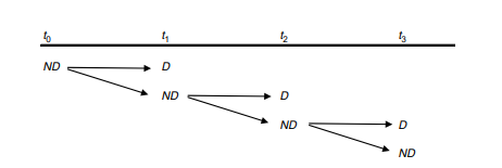
We discretize the remaining time to maturity of the CDS, i.e., the time interval $[0 \mathrm{~T}]$, into $n$ intervals with equal distance $\Delta t$ between the grid points. For $n=3$, Figure $1.6$ pictures the evolution of the default status of the reference bond.
At $t_{0}$ the company is alive (nondefault, $N D$ ) with probability 1 . At $t_{1}$, the company can default $(D)$ or survive $(N D)$. If it defaults, this state remains the same for the future. If the firm did not default, the tree will further branch out with two possible states ( $D$ and $N D$ at $t_{2}$ ). Default at any $t_{i}$ acts as an “absorbing state” for the rest of the tree.
Let us refer back to our example in Table 1.1, where the cash flows for the buyer of a 3 year CDS with annual payments were summarized. Time was discretized in $n=6$ steps of $0.5$ years. Bankruptcy can occur on every node (column). In case of $N D$ at time $T$, the last payment occurs at $t_{4}$ or at $T$ depending on the contract specification.
In case of $D$, the payment of the premium payments stops but a last accrued premium may contractually be due at the time of default. This accrued fee is netted with the payment the protection seller has to pay in case of $D$. For the buyer, the $t_{3}$-value of the settlement of the CDS is $F(1-R)$. Depending on the contract specifications the par value can be augmented with the accrued interest from $t_{2}$ to $t_{3}$. In most general terms, the payment becomes $(F+A I)(1-R)-A F$.
金融代写|金融数学作业代写Financial Mathematics代考|Default Probabilities
The default status tree (Figure $1.6$ ) neglected the probabilities. The definition of the various default and survival probabilities makes the literature not very transparent. Deciphering notation is most of the time the hardest part of understanding the model.
First let us define the probability of default at each node in the tree, $p_{(i)}$, as the probability to default during period $i$. The firm still was alive at $t_{i-1}$, it defaults at $t_{i}$. Whenever the default probabilities are kept constant over time, such as in Figure 1.7, we will drop the subscript. In Figure $1.7 p=5 \%$.
These default probabilities define a number of conditional probabilities characterizing the various states of the default process.
For the first period the marginal probabilities apply:
$$
\begin{gathered}
P\left(D_{1}\right)=p_{(1)}=5 \% \
P\left(N D_{1}\right)=\left(1-p_{(1)}\right)=95 \%
\end{gathered}
$$
For the second period,
$$
\begin{gathered}
P\left(D_{2} \mid N D_{1}\right)=\left(1-p_{(1)}\right) p_{(2)}=4.75 \% \
P\left(N D_{2} \mid N D_{1}\right)=\left(1-p_{(1)}\right)\left(1-p_{(2)}\right)=90.25 \%
\end{gathered}
$$
For the third period, we get
$$
\begin{gathered}
P\left(D_{3} \mid N D_{2}\right)=\left(1-p_{(1)}\right)\left(1-p_{(2)}\right) p_{(3)}=4.51 \% \
P\left(N D_{3} \mid N D_{2}\right)=\left(1-p_{(1)}\right)\left(1-p_{(2)}\right)\left(1-p_{(3)}\right)=85.74 \%
\end{gathered}
$$
Two series of probabilities emerge:
- On the one hand, we find the probabilities of survival until time $t_{i}$, which we will denote $\pi_{i}: 95 \%, 90.25 \%$, and $85.74 \%$.
- On the other hand, we obtain the probability of default at time $t_{i}$, conditional upon survival until the previous period: $5 \%, 4.75 \%$, and $4.51 \%$. We will denote these probabilities by $p_{i}$.
In general, we can express these conditional probabilities for $t_{i}$ as
$$
\left{\begin{array}{l}
p_{1}=p_{(1)} \
p_{i}=P\left(D_{i} \mid N D_{i-1}\right)=p_{(i)} \prod_{j=2}^{i}\left(1-p_{(j-1)}\right) \quad \text { for } i=2,3, \ldots, n \
\pi_{i}=P\left(N D_{i} \mid N D_{i-1}\right)=\prod_{j=1}^{i}\left(1-p_{(j)}\right) \quad \text { for } i=1,2, \ldots, n
\end{array}\right.
$$
If the default probability is constant over the tree, these formulas for $i=1,2, \ldots, n$ collapse to
$$
\begin{aligned}
&p_{i}=P\left(D_{i} \mid N D_{i-1}\right)=p(1-p)^{i-1} \
&\pi_{i}=P\left(N D_{i} \mid N D_{i-1}\right)=(1-p)^{i}
\end{aligned}
$$
Note that the following relationships hold:
- Probability of survival until time $t_{i}$ is equal to 1 minus the sum of the conditional probabilities of default in the previous periods: $\pi_{i}=1-\sum_{j=1}^{i} p_{j}$.
- Probability of survival until time $t_{i}$ is equal to the probability of survival until the previous time minus the conditional probability to default in period $i: \pi_{i}=\pi_{i-1}-p_{i}$.
- Probability to survival until time $t_{i}$ is equal to the probability of survival until the previous period multiplied by the factor 1 minus the default probability (given that the default probability is constant): $\pi_{i}=\pi_{i-1}(1-p)$ or even more general $\pi_{i}=\pi_{i-j}$ $(1-p)^{j}$ with $j<i$ and $j \in N$.
金融代写|金融数学作业代写Financial Mathematics代考|Risk Neutral Pricing of the CDS
The periodic premium payments are generally labeled in the literature as the floating leg. The contingent terminal payment is known as the fixed leg of the CDS.
1.5.5.1 Under the Discrete Default Process
1.5.5.1.1 Floating Leg At the payment dates $t_{g} t_{2 g}, \ldots, t_{n}$ the protection buyer pays the premium $P=s F(g \Delta t$ ), until (and not including) default.
The expected payment for time $t_{i}$, seen today, is $P\left(N D_{i} \mid N D_{i-1}\right) P+P\left(D_{i} \mid N D_{i-1}\right) 0=\pi_{i} P$. Consequently, the present value of the expected payments is $\sum_{i=1}^{n / g} d f_{i g} \pi_{i g} P$ where $d f_{i}$ denotes the discount factor for the time $t_{\text {ig }}$ cash flow.
- Note that the discount function can be expressed in various ways:
- Cheng (2001) uses the general zero bond price formulation: $B\left(t_{0}, t_{n}\right)$ i.e., the time $t_{0}$ value of a default free zero bond maturing at $t_{n}$.
- Brooks and Yan (1998) use simple one period forward rates: $d f_{i}=\frac{d f_{i-1}}{1+r_{w-1} \times W_{i}}$. NAD is the number of accrued days and NTD the total number of days, defining the applicable day count convention.
- Continuous interest rates would yield: $\mathrm{e}^{-r_{i} t_{i}}$.
- Scott (1998), Aonuma and Nakagawa (1998), Houweling and Vorst (2005), Longstaff, Mithal and Neis (2005) use the stochastic interest formulation: $\mathrm{e}^{-\int_{0}^{t} r(u) \mathrm{d} u}$.Also with the probabilities we can juggle a bit. Note that, as Figure $1.8$ illustrates, the survival probability, $\pi_{b}, i<n$ equals the sum of the survival probability at the end of the contract, $\pi_{n}$, plus the sum of the probabilities of defaulting between $t_{i}$ and $t_{n}$.
- $$
- \begin{gathered}
- \pi_{i}=\pi_{n}+\sum_{j=i}^{n} p_{j} \
- \sum_{i=1}^{n / g} d f_{i g} \pi_{i g} P \text { then becomes } \sum_{i=1}^{n / g} d f_{i g}\left(\pi_{n / g}+\sum_{j=i+1}^{n / g} p_{j}\right) P
- \end{gathered}
- $$
- which is a formulation Brooks and Yan (1998) use.
金融数学代写
金融代写|金融数学作业代写Financial Mathematics代考|Default Status Tree
如今,金融产品的估值是在风险中性概率测度下的预期现金流量的折现值。我们可以使用 Jarrow 和 Turnbull (1995) 中的风险中性估值方法以无风险利率对支付进行贴现。这意味着风险中性世界中的违约概率是相关的。
我们将CDS的剩余到期时间离散化,即时间间隔[0 吨], 进入n等距间隔Δ吨网格点之间。为了n=3, 数字1.6图片显示了参考债券违约状态的演变。
在吨0公司还活着(非违约,ñD) 概率为 1 。在吨1, 公司可以违约(D)或生存(ñD). 如果它默认,则此状态在未来保持不变。如果公司没有违约,树将进一步分支出两种可能的状态(D和ñD在吨2)。任意默认吨一世充当树的其余部分的“吸收状态”。
让我们回顾一下表 1.1 中的示例,其中汇总了购买 3 年期 CDS 且按年支付的现金流量。时间被离散化为n=6的步骤0.5年。每个节点(列)都可能发生破产。的情况下ñD有时吨,最后一次付款发生在吨4或吨取决于合同规范。
的情况下D,保费支付停止,但最后应计的保费可能在违约时到期。该应计费用与保护卖方在以下情况下必须支付的款项相抵D. 对于买家来说,吨3-CDS 的结算价值为F(1−R). 根据合约规格,面值可随应计利息增加吨2到吨3. 在最一般的情况下,付款变成(F+一种一世)(1−R)−一种F.
金融代写|金融数学作业代写Financial Mathematics代考|Default Probabilities
默认状态树(图1.6) 忽略了概率。各种违约和生存概率的定义使得文献不是很透明。在大多数情况下,解读符号是理解模型最难的部分。
首先让我们定义树中每个节点的违约概率,p(一世),作为期间违约的概率一世. 公司还活着吨一世−1,默认为吨一世. 每当默认概率随时间保持不变时,例如在图 1.7 中,我们将删除下标。如图1.7p=5%.
这些默认概率定义了许多表征默认过程的各种状态的条件概率。
对于第一个时期,边际概率适用:
磷(D1)=p(1)=5% 磷(ñD1)=(1−p(1))=95%
第二期,
磷(D2∣ñD1)=(1−p(1))p(2)=4.75% 磷(ñD2∣ñD1)=(1−p(1))(1−p(2))=90.25%
对于第三个时期,我们得到
磷(D3∣ñD2)=(1−p(1))(1−p(2))p(3)=4.51% 磷(ñD3∣ñD2)=(1−p(1))(1−p(2))(1−p(3))=85.74%
出现了两个系列的概率:
- 一方面,我们发现直到时间的生存概率吨一世, 我们将表示圆周率一世:95%,90.25%, 和85.74%.
- 另一方面,我们获得了违约概率吨一世, 以生存到前一时期为条件:5%,4.75%, 和4.51%. 我们将这些概率表示为p一世.
一般来说,我们可以将这些条件概率表示为吨一世作为
$$
\left{p1=p(1) p一世=磷(D一世∣ñD一世−1)=p(一世)∏j=2一世(1−p(j−1)) 为了 一世=2,3,…,n 圆周率一世=磷(ñD一世∣ñD一世−1)=∏j=1一世(1−p(j)) 为了 一世=1,2,…,n\对。
一世F吨H和d和F一种在l吨pr这b一种b一世l一世吨是一世sC这ns吨一种n吨这在和r吨H和吨r和和,吨H和s和F这r米在l一种sF这r$一世=1,2,…,n$C这ll一种ps和吨这
p一世=磷(D一世∣ñD一世−1)=p(1−p)一世−1 圆周率一世=磷(ñD一世∣ñD一世−1)=(1−p)一世
$$
请注意,以下关系成立:
- 直到时间的生存概率吨一世等于 1 减去前期违约条件概率的总和:圆周率一世=1−∑j=1一世pj.
- 直到时间的生存概率吨一世等于直到前一次的生存概率减去该期间违约的条件概率一世:圆周率一世=圆周率一世−1−p一世.
- 生存到时间的概率吨一世等于直到前一时期的生存概率乘以因子 1 减去违约概率(假设违约概率是常数):圆周率一世=圆周率一世−1(1−p)甚至更一般圆周率一世=圆周率一世−j (1−p)j和j<一世和j∈ñ.
金融代写|金融数学作业代写Financial Mathematics代考|Risk Neutral Pricing of the CDS
定期支付的保费在文献中通常被标记为浮动腿。或有终端支付被称为 CDS 的固定腿。
1.5.5.1 在离散违约过程下
1.5.5.1.1 浮动腿 在付款日吨G吨2G,…,吨n保护买方支付保费磷=sF(GΔ吨),直到(不包括)默认值。
预期的时间付款吨一世,今天看到的是磷(ñD一世∣ñD一世−1)磷+磷(D一世∣ñD一世−1)0=圆周率一世磷. 因此,预期付款的现值为∑一世=1n/GdF一世G圆周率一世G磷在哪里dF一世表示该时间的折扣因子吨ig 现金周转。
- 请注意,折扣函数可以用多种方式表示:
- Cheng (2001) 使用一般的零债券价格公式:乙(吨0,吨n)即时间吨0到期的违约免费零债券的价值吨n.
- Brooks and Yan (1998) 使用简单的一期远期汇率:dF一世=dF一世−11+r在−1×在一世. NAD 是累计天数,NTD 是总天数,定义了适用的天数计算惯例。
- 连续利率将产生:和−r一世吨一世.
- Scott (1998)、Aonuma 和 Nakagawa (1998)、Houweling 和 Vorst (2005)、Longstaff、Mithal 和 Neis (2005) 使用随机利率公式:和−∫0吨r(在)d在.另外,我们可以稍微调整一下概率。请注意,如图1.8说明,生存概率,圆周率b,一世<n等于合约结束时的生存概率之和,圆周率n,加上之间违约概率的总和吨一世和吨n.
- $$
- \开始{聚集}
- \pi_{i}=\pi_{n}+\sum_{j=i}^{n} p_{j} \
- \sum_{i=1}^{n / g} d f_{ig} \pi_{ig} P \text { 然后变成 } \sum_{i=1}^{n / g} d f_{ig}\left (\pi_{n / g}+\sum_{j=i+1}^{n / g} p_{j}\right) P
- \结束{聚集}
- $$
- 这是 Brooks 和 Yan (1998) 使用的公式。

统计代写请认准statistics-lab™. statistics-lab™为您的留学生涯保驾护航。
金融工程代写
金融工程是使用数学技术来解决金融问题。金融工程使用计算机科学、统计学、经济学和应用数学领域的工具和知识来解决当前的金融问题,以及设计新的和创新的金融产品。
非参数统计代写
非参数统计指的是一种统计方法,其中不假设数据来自于由少数参数决定的规定模型;这种模型的例子包括正态分布模型和线性回归模型。
广义线性模型代考
广义线性模型(GLM)归属统计学领域,是一种应用灵活的线性回归模型。该模型允许因变量的偏差分布有除了正态分布之外的其它分布。
术语 广义线性模型(GLM)通常是指给定连续和/或分类预测因素的连续响应变量的常规线性回归模型。它包括多元线性回归,以及方差分析和方差分析(仅含固定效应)。
有限元方法代写
有限元方法(FEM)是一种流行的方法,用于数值解决工程和数学建模中出现的微分方程。典型的问题领域包括结构分析、传热、流体流动、质量运输和电磁势等传统领域。
有限元是一种通用的数值方法,用于解决两个或三个空间变量的偏微分方程(即一些边界值问题)。为了解决一个问题,有限元将一个大系统细分为更小、更简单的部分,称为有限元。这是通过在空间维度上的特定空间离散化来实现的,它是通过构建对象的网格来实现的:用于求解的数值域,它有有限数量的点。边界值问题的有限元方法表述最终导致一个代数方程组。该方法在域上对未知函数进行逼近。[1] 然后将模拟这些有限元的简单方程组合成一个更大的方程系统,以模拟整个问题。然后,有限元通过变化微积分使相关的误差函数最小化来逼近一个解决方案。
tatistics-lab作为专业的留学生服务机构,多年来已为美国、英国、加拿大、澳洲等留学热门地的学生提供专业的学术服务,包括但不限于Essay代写,Assignment代写,Dissertation代写,Report代写,小组作业代写,Proposal代写,Paper代写,Presentation代写,计算机作业代写,论文修改和润色,网课代做,exam代考等等。写作范围涵盖高中,本科,研究生等海外留学全阶段,辐射金融,经济学,会计学,审计学,管理学等全球99%专业科目。写作团队既有专业英语母语作者,也有海外名校硕博留学生,每位写作老师都拥有过硬的语言能力,专业的学科背景和学术写作经验。我们承诺100%原创,100%专业,100%准时,100%满意。
随机分析代写
随机微积分是数学的一个分支,对随机过程进行操作。它允许为随机过程的积分定义一个关于随机过程的一致的积分理论。这个领域是由日本数学家伊藤清在第二次世界大战期间创建并开始的。
时间序列分析代写
随机过程,是依赖于参数的一组随机变量的全体,参数通常是时间。 随机变量是随机现象的数量表现,其时间序列是一组按照时间发生先后顺序进行排列的数据点序列。通常一组时间序列的时间间隔为一恒定值(如1秒,5分钟,12小时,7天,1年),因此时间序列可以作为离散时间数据进行分析处理。研究时间序列数据的意义在于现实中,往往需要研究某个事物其随时间发展变化的规律。这就需要通过研究该事物过去发展的历史记录,以得到其自身发展的规律。
回归分析代写
多元回归分析渐进(Multiple Regression Analysis Asymptotics)属于计量经济学领域,主要是一种数学上的统计分析方法,可以分析复杂情况下各影响因素的数学关系,在自然科学、社会和经济学等多个领域内应用广泛。
MATLAB代写
MATLAB 是一种用于技术计算的高性能语言。它将计算、可视化和编程集成在一个易于使用的环境中,其中问题和解决方案以熟悉的数学符号表示。典型用途包括:数学和计算算法开发建模、仿真和原型制作数据分析、探索和可视化科学和工程图形应用程序开发,包括图形用户界面构建MATLAB 是一个交互式系统,其基本数据元素是一个不需要维度的数组。这使您可以解决许多技术计算问题,尤其是那些具有矩阵和向量公式的问题,而只需用 C 或 Fortran 等标量非交互式语言编写程序所需的时间的一小部分。MATLAB 名称代表矩阵实验室。MATLAB 最初的编写目的是提供对由 LINPACK 和 EISPACK 项目开发的矩阵软件的轻松访问,这两个项目共同代表了矩阵计算软件的最新技术。MATLAB 经过多年的发展,得到了许多用户的投入。在大学环境中,它是数学、工程和科学入门和高级课程的标准教学工具。在工业领域,MATLAB 是高效研究、开发和分析的首选工具。MATLAB 具有一系列称为工具箱的特定于应用程序的解决方案。对于大多数 MATLAB 用户来说非常重要,工具箱允许您学习和应用专业技术。工具箱是 MATLAB 函数(M 文件)的综合集合,可扩展 MATLAB 环境以解决特定类别的问题。可用工具箱的领域包括信号处理、控制系统、神经网络、模糊逻辑、小波、仿真等。