如果你也在 怎样代写优化算法optimisation algorithms这个学科遇到相关的难题，请随时右上角联系我们的24/7代写客服。

优化算法是一个通过比较各种解决方案来反复执行的程序，直到找到一个最佳或满意的解决方案。随着计算机的出现，优化已成为计算机辅助设计活动的一部分。

statistics-lab™ 为您的留学生涯保驾护航 在代写优化算法optimisation algorithms方面已经树立了自己的口碑, 保证靠谱, 高质且原创的统计Statistics代写服务。我们的专家在代写优化算法optimisation algorithms代写方面经验极为丰富，各种代写优化算法optimisation algorithms相关的作业也就用不着说。

我们提供的优化算法optimisation algorithms及其相关学科的代写，服务范围广, 其中包括但不限于:

• Statistical Inference 统计推断
• Statistical Computing 统计计算
• Advanced Probability Theory 高等楖率论
• Advanced Mathematical Statistics 高等数理统计学
• (Generalized) Linear Models 广义线性模型
• Statistical Machine Learning 统计机器学习
• Longitudinal Data Analysis 纵向数据分析
• Foundations of Data Science 数据科学基础

• Statistical Inference 统计推断
• Statistical Computing 统计计算
• Advanced Probability Theory 高等楖率论
• Advanced Mathematical Statistics 高等数理统计学
• (Generalized) Linear Models 广义线性模型
• Statistical Machine Learning 统计机器学习
• Longitudinal Data Analysis 纵向数据分析
• Foundations of Data Science 数据科学基础

数学代写|优化算法作业代写optimisation algorithms代考|The Problem

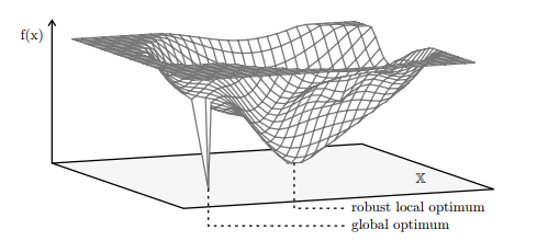
Definition 5 (Overfitting). Overfitting is the emergence of an overly complicated model (solution candidate) in an optimization process resulting from the effort to provide the best results for as much of the available training data as possible $[64,80,190,202]$.

A model (solution candidate) $m \in X$ created with a finite set of training data is considered to be overfitted if a less complicated, alternative model

$m^{\prime} \in X$ exists which has a smaller error for the set of all possible (maybe even infinitely many), available, or (theoretically) producible data samples. This model $m^{\prime}$ may, however, have a larger error in the training data.

The phenomenon of overfitting is best known and can often be encountered in the field of artificial neural networks or in curve fitting $[124,128,181,191$, 211]. The latter means that we have a set $A$ of $n$ training data samples $\left(x_{i}, y_{i}\right)$ and want to find a function $f$ that represents these samples as well as possible, i.e., $f\left(x_{i}\right)=y_{i} \forall\left(x_{i}, y_{i}\right) \in A$.

There exists exactly one polynomial of the degree $n-1$ that fits to each such training data and goes through all its points. Hence, when only polynomial regression is performed, there is exactly one perfectly fitting function of minimal degree. Nevertheless, there will also be an infinite number of polynomials with a higher degree than $n-1$ that also match the sample data perfectly. Such results would be considered as overfitted.

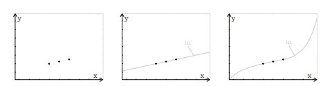
In Fig. 9, we have sketched this problem. The function $f_{1}(x)=x$ shown in Fig. 9.b has been sampled three times, as sketched in Fig. 9.a. There exists no other polynomial of a degree of two or less that fits to these samples than $f_{1}$. Optimizers, however, could also find overfitted polynomials of a higher degree such as $f_{2}$ which also match the data, as shown in Fig. 9.c. Here, $f_{2}$ plays the role of the overly complicated model $m$ which will perform as good as the simpler model $m^{\prime}$ when tested with the training sets only, but will fail to deliver good results for all other input data.

数学代写|优化算法作业代写optimisation algorithms代考|Countermeasures

There exist multiple techniques that can be utilized in order to prevent overfitting to a certain degree. It is most efficient to apply multiple such techniques together in order to achieve best results.

A very simple approach is to restrict the problem space $X$ in a way that only solutions up to a given maximum complexity can be found. In terms of function fitting, this could mean limiting the maximum degree of the polynomials to be tested. Furthermore, the functional objective functions which solely concentrate on the error of the solution candidates should be augmented by penalty terms and non-functional objective functions putting pressure in the direction of small and simple models $[64,116]$.

Large sets of sample data, although slowing down the optimization process, may improve the generalization capabilities of the derived solutions. If arbitrarily many training datasets or training scenarios can be generated, there are two approaches which work against overfitting:

1. The first method is to use a new set of (randomized) scenarios for each evaluation of a solution candidate. The resulting objective values may differ

largely even if the same individual is evaluated twice in a row, introducing incoherence and ruggedness into the fitness landscape.

2. At the beginning of each iteration of the optimizer, a new set of (randomized) scenarios is generated which is used for all individual evaluations during that iteration. This method leads to objective values which can be compared without bias.

In both cases it is helpful to use more than one training sample or scenario per evaluation and to set the resulting objective value to the average (or better median) of the outcomes. Otherwise, the fluctuations of the objective values between the iterations will be very large, making it hard for the optimizers to follow a stable gradient for multiple steps.

Another simple method to prevent overfitting is to limit the runtime of the optimizers [190]. It is commonly assumed that learning processes normally first find relatively general solutions which subsequently begin to overfit because the noise “is learned”, too.

For the same reason, some algorithms allow to decrease the rate at which the solution candidates are modified by time. Such a decay of the learning rate makes overfitting less likely.

If only one finite set of data samples is available for training/optimization, it is common practice to separate it into a set of training data $A_{t}$ and a set of test cases $A_{c}$. During the optimization process, only the training data is used. The resulting solutions are tested with the test cases afterwards. If their behavior is significantly worse when applied to $A_{c}$ than when applied to $A_{t}$, they are probably overfitted.

The same approach can be used to detect when the optimization process should be stopped. The best known solution candidates can be checked with the test cases in each iteration without influencing their objective values which solely depend on the training data. If their performance on the test cases begins to decrease, there are no benefits in letting the optimization process continue any further.

数学代写|优化算法作业代写optimisation algorithms代考|The Problem

Oversimplification (also called overgeneralization) is the opposite of overfitting. Whereas overfitting denotes the emergence of overly-complicated solution candidates, oversimplified solutions are not complicated enough. Although they represent the training samples used during the optimization process seemingly well, they are rough overgeneralizations which fail to provide good results for cases not part of the training.

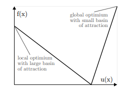
A common cause for oversimplification is sketched in Fig. 11: The training sets only represent a fraction of the set of possible inputs. As this is normally the case, one should always be aware that such an incomplete coverage may fail to represent some of the dependencies and characteristics of the data.

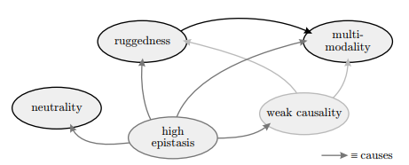
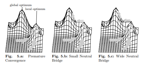
which then may lead to oversimplified solutions. Another possible reason is that ruggedness, deceptiveness, too much neutrality, or high epistasis in the fitness landscape may lead to premature convergence and prevent the optimizer from surpassing a certain quality of the solution candidates. It then cannot completely adapt them even if the training data perfectly represents the sampled process. A third cause is that a problem space which does not include the correct solution was chosen.

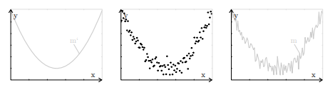
Fig. 11.a shows a cubic function. Since it is a polynomial of degree three, four sample points are needed for its unique identification. Maybe not knowing this, only three samples have been provided in Fig. 11.b. By doing so, some vital characteristics of the function are lost. Fig. 11.c depicts a square function – the polynomial of the lowest degree that fits exactly to these samples. Although it is a perfect match, this function does not touch any other point on the original cubic curve and behaves totally differently at the lower parameter area.

However, even if we had included point $P$ in our training data, it would still be possible that the optimization process would yield Fig. 11.c as a result. Having training data that correctly represents the sampled system does not mean that the optimizer is able to find a correct solution with perfect fitness – the other, previously discussed problematic phenomena can prevent it from doing so. Furthermore, if it was not known that the system which was to be modeled by the optimization process can best be represented by a polynomial of the third degree, one could have limited the problem space $\mathbb{X}$ to polynomials of degree two and less. Then, the result would likely again be something like Fig. 11.c, regardless of how many training samples are used.

优化算法代考

数学代写|优化算法作业代写optimisation algorithms代考|The Problem

定义 5（过拟合）。过度拟合是由于努力为尽可能多的可用训练数据提供最佳结果而导致的优化过程中出现的过于复杂的模型（候选解决方案）[64,80,190,202].

模型（候选解决方案）米∈X如果使用不太复杂的替代模型，则使用有限的训练数据集创建的模型被认为是过拟合的

米′∈X对于所有可能（甚至无限多）、可用或（理论上）可生产的数据样本的集合，存在较小的误差。该型号米′但是，可能在训练数据中有较大的误差。

过拟合现象最为人所知，在人工神经网络领域或曲线拟合中经常会遇到[124,128,181,191, 211]。后者意味着我们有一个集合一种的n训练数据样本(X一世,是一世)并想找到一个功能F尽可能好地代表这些样本，即F(X一世)=是一世∀(X一世,是一世)∈一种.

只存在一个次数的多项式n−1适合每个这样的训练数据并贯穿其所有要点。因此，当只进行多项式回归时，恰好有一个最小度的完美拟合函数。尽管如此，也会有无数个多项式的次数高于n−1这也与样本数据完美匹配。这样的结果将被视为过度拟合。

在图 9 中，我们勾画了这个问题。功能F1(X)=X如图 9.a 所示，图 9.b 所示已被采样 3 次。不存在适合这些样本的二次或更少次数的多项式F1. 然而，优化器也可以找到更高程度的过度拟合多项式，例如F2这也与数据匹配，如图 9.c 所示。这里，F2扮演过于复杂的模型米这将与更简单的模型一样好米′当仅使用训练集进行测试时，将无法为所有其他输入数据提供良好的结果。

数学代写|优化算法作业代写optimisation algorithms代考|Countermeasures

有多种技术可以用来在一定程度上防止过度拟合。将多种此类技术一起应用以获得最佳结果是最有效的。

一个非常简单的方法是限制问题空间X以某种方式只能找到达到给定最大复杂性的解决方案。在函数拟合方面，这可能意味着限制要测试的多项式的最大次数。此外，仅关注候选解决方案误差的功能性目标函数应通过惩罚项和非功能性目标函数来增强，从而向小型和简单模型的方向施加压力[64,116].

大量样本数据集虽然减慢了优化过程，但可能会提高派生解决方案的泛化能力。如果可以生成任意多个训练数据集或训练场景，则有两种方法可以防止过拟合：

1. 第一种方法是对候选解决方案的每次评估使用一组新的（随机）场景。产生的客观值可能不同

即使同一个人连续两次被评估，也会在很大程度上将不连贯性和坚固性引入到健身环境中。

2. 在优化器的每次迭代开始时，会生成一组新的（随机）场景，用于该迭代期间的所有单独评估。这种方法产生的客观值可以在没有偏差的情况下进行比较。

在这两种情况下，每次评估使用多个训练样本或场景并将结果目标值设置为结果的平均值（或更好的中位数）是有帮助的。否则，迭代之间的目标值波动将非常大，使得优化器难以在多个步骤中遵循稳定的梯度。

另一种防止过拟合的简单方法是限制优化器的运行时间[190]。通常假设学习过程通常首先找到相对一般的解决方案，然后由于噪声“被学习”而开始过度拟合。

出于同样的原因，一些算法允许降低候选解决方案随时间修改的速率。学习率的这种衰减使得过拟合的可能性降低。

如果只有一组有限的数据样本可用于训练/优化，通常的做法是将其分成一组训练数据一种吨和一组测试用例一种C. 在优化过程中，仅使用训练数据。之后使用测试用例对生成的解决方案进行测试。如果他们的行为在应用于一种C比应用于一种吨，它们可能是过拟合的。

可以使用相同的方法来检测何时应该停止优化过程。可以在每次迭代中使用测试用例检查最知名的候选解决方案，而不会影响其仅取决于训练数据的目标值。如果它们在测试用例上的性能开始下降，那么让优化过程继续下去没有任何好处。

数学代写|优化算法作业代写optimisation algorithms代考|The Problem

过度简化（也称为过度泛化）与过度拟合相反。虽然过度拟合表示出现了过于复杂的候选解决方案，但过于简单的解决方案还不够复杂。尽管它们似乎很好地代表了优化过程中使用的训练样本，但它们是粗略的过度概括，无法为不属于训练的情况提供良好的结果。

图 11 概述了过度简化的一个常见原因：训练集仅代表可能输入集的一小部分。由于通常情况如此，因此应始终注意，这种不完整的覆盖范围可能无法代表数据的某些依赖性和特征。

这可能会导致解决方案过于简单。另一个可能的原因是，适应度环境中的坚固性、欺骗性、过多的中立性或高上位性可能导致过早收敛并阻止优化器超过解决方案候选者的一定质量。即使训练数据完美地代表了采样过程，它也无法完全适应它们。第三个原因是选择了不包括正确解决方案的问题空间。

图 11.a 显示了一个三次函数。由于它是一个三阶多项式，因此需要四个样本点来唯一识别。也许不知道这一点，图 11.b 中只提供了三个样本。这样做会丢失该功能的一些重要特征。图 11.c 描绘了一个平方函数——与这些样本完全吻合的最低阶多项式。虽然是完美匹配，但此函数不会触及原始三次曲线上的任何其他点，并且在较低参数区域的行为完全不同。

但是，即使我们包含了点磷在我们的训练数据中，优​​化过程仍然有可能产生图 11.c 的结果。拥有正确表示采样系统的训练数据并不意味着优化器能够找到具有完美适应度的正确解决方案——另一个先前讨论过的有问题的现象可能会阻止它这样做。此外，如果不知道要通过优化过程建模的系统可以用三次多项式最好地表示，那么可能会限制问题空间X为二次及以下的多项式。然后，无论使用多少训练样本，结果都可能再次类似于图 11.c。

统计代写请认准statistics-lab™. statistics-lab™为您的留学生涯保驾护航。

金融工程代写

金融工程是使用数学技术来解决金融问题。金融工程使用计算机科学、统计学、经济学和应用数学领域的工具和知识来解决当前的金融问题，以及设计新的和创新的金融产品。

非参数统计代写

非参数统计指的是一种统计方法，其中不假设数据来自于由少数参数决定的规定模型；这种模型的例子包括正态分布模型和线性回归模型。

广义线性模型代考

广义线性模型（GLM）归属统计学领域，是一种应用灵活的线性回归模型。该模型允许因变量的偏差分布有除了正态分布之外的其它分布。

术语 广义线性模型（GLM）通常是指给定连续和/或分类预测因素的连续响应变量的常规线性回归模型。它包括多元线性回归，以及方差分析和方差分析（仅含固定效应）。

有限元方法代写

有限元方法（FEM）是一种流行的方法，用于数值解决工程和数学建模中出现的微分方程。典型的问题领域包括结构分析、传热、流体流动、质量运输和电磁势等传统领域。

有限元是一种通用的数值方法，用于解决两个或三个空间变量的偏微分方程（即一些边界值问题）。为了解决一个问题，有限元将一个大系统细分为更小、更简单的部分，称为有限元。这是通过在空间维度上的特定空间离散化来实现的，它是通过构建对象的网格来实现的：用于求解的数值域，它有有限数量的点。边界值问题的有限元方法表述最终导致一个代数方程组。该方法在域上对未知函数进行逼近。[1] 然后将模拟这些有限元的简单方程组合成一个更大的方程系统，以模拟整个问题。然后，有限元通过变化微积分使相关的误差函数最小化来逼近一个解决方案。

tatistics-lab作为专业的留学生服务机构，多年来已为美国、英国、加拿大、澳洲等留学热门地的学生提供专业的学术服务，包括但不限于Essay代写，Assignment代写，Dissertation代写，Report代写，小组作业代写，Proposal代写，Paper代写，Presentation代写，计算机作业代写，论文修改和润色，网课代做，exam代考等等。写作范围涵盖高中，本科，研究生等海外留学全阶段，辐射金融，经济学，会计学，审计学，管理学等全球99%专业科目。写作团队既有专业英语母语作者，也有海外名校硕博留学生，每位写作老师都拥有过硬的语言能力，专业的学科背景和学术写作经验。我们承诺100%原创，100%专业，100%准时，100%满意。

随机分析代写

随机微积分是数学的一个分支，对随机过程进行操作。它允许为随机过程的积分定义一个关于随机过程的一致的积分理论。这个领域是由日本数学家伊藤清在第二次世界大战期间创建并开始的。

时间序列分析代写

随机过程，是依赖于参数的一组随机变量的全体，参数通常是时间。 随机变量是随机现象的数量表现，其时间序列是一组按照时间发生先后顺序进行排列的数据点序列。通常一组时间序列的时间间隔为一恒定值（如1秒，5分钟，12小时，7天，1年），因此时间序列可以作为离散时间数据进行分析处理。研究时间序列数据的意义在于现实中，往往需要研究某个事物其随时间发展变化的规律。这就需要通过研究该事物过去发展的历史记录，以得到其自身发展的规律。

回归分析代写

多元回归分析渐进（Multiple Regression Analysis Asymptotics）属于计量经济学领域，主要是一种数学上的统计分析方法，可以分析复杂情况下各影响因素的数学关系，在自然科学、社会和经济学等多个领域内应用广泛。

MATLAB代写

MATLAB 是一种用于技术计算的高性能语言。它将计算、可视化和编程集成在一个易于使用的环境中，其中问题和解决方案以熟悉的数学符号表示。典型用途包括：数学和计算算法开发建模、仿真和原型制作数据分析、探索和可视化科学和工程图形应用程序开发，包括图形用户界面构建MATLAB 是一个交互式系统，其基本数据元素是一个不需要维度的数组。这使您可以解决许多技术计算问题，尤其是那些具有矩阵和向量公式的问题，而只需用 C 或 Fortran 等标量非交互式语言编写程序所需的时间的一小部分。MATLAB 名称代表矩阵实验室。MATLAB 最初的编写目的是提供对由 LINPACK 和 EISPACK 项目开发的矩阵软件的轻松访问，这两个项目共同代表了矩阵计算软件的最新技术。MATLAB 经过多年的发展，得到了许多用户的投入。在大学环境中，它是数学、工程和科学入门和高级课程的标准教学工具。在工业领域，MATLAB 是高效研究、开发和分析的首选工具。MATLAB 具有一系列称为工具箱的特定于应用程序的解决方案。对于大多数 MATLAB 用户来说非常重要，工具箱允许您学习和应用专业技术。工具箱是 MATLAB 函数（M 文件）的综合集合，可扩展 MATLAB 环境以解决特定类别的问题。可用工具箱的领域包括信号处理、控制系统、神经网络、模糊逻辑、小波、仿真等。

R语言代写	问卷设计与分析代写
PYTHON代写	回归分析与线性模型代写
MATLAB代写	方差分析与试验设计代写
STATA代写	机器学习/统计学习代写
SPSS代写	计量经济学代写
EVIEWS代写	时间序列分析代写
EXCEL代写	深度学习代写
SQL代写	各种数据建模与可视化代写

如果你也在 怎样代写优化算法optimisation algorithms这个学科遇到相关的难题，请随时右上角联系我们的24/7代写客服。

优化算法是一个通过比较各种解决方案来反复执行的程序，直到找到一个最佳或满意的解决方案。随着计算机的出现，优化已成为计算机辅助设计活动的一部分。

statistics-lab™ 为您的留学生涯保驾护航 在代写优化算法optimisation algorithms方面已经树立了自己的口碑, 保证靠谱, 高质且原创的统计Statistics代写服务。我们的专家在代写优化算法optimisation algorithms代写方面经验极为丰富，各种代写优化算法optimisation algorithms相关的作业也就用不着说。

我们提供的优化算法optimisation algorithms及其相关学科的代写，服务范围广, 其中包括但不限于:

• Statistical Inference 统计推断
• Statistical Computing 统计计算
• Advanced Probability Theory 高等楖率论
• Advanced Mathematical Statistics 高等数理统计学
• (Generalized) Linear Models 广义线性模型
• Statistical Machine Learning 统计机器学习
• Longitudinal Data Analysis 纵向数据分析
• Foundations of Data Science 数据科学基础

• Statistical Inference 统计推断
• Statistical Computing 统计计算
• Advanced Probability Theory 高等楖率论
• Advanced Mathematical Statistics 高等数理统计学
• (Generalized) Linear Models 广义线性模型
• Statistical Machine Learning 统计机器学习
• Longitudinal Data Analysis 纵向数据分析
• Foundations of Data Science 数据科学基础

数学代写|优化算法作业代写optimisation algorithms代考|Introduction – Noise

In the context of optimization, three types of noise can be distinguished. The first form is noise in the training data used as basis for learning (i). In many applications of machine learning or optimization where a model $m$ for a given system is to be learned, data samples including the input of the system and its measured response are used for training. Some typical examples of situations where training data is the basis for the objective function evaluation are

• the usage of global optimization for building classifiers (for example for predicting buying behavior using data gathered in a customer survey for training).
• the usage of simulations for determining the objective values in Genetic Programming (here, the simulated scenarios correspond to training cases), and
• the fitting of mathematical functions to $(x, y)$-data samples (with artificial neural networks or symbolic regression, for instance).

Since no measurement device is $100 \%$ accurate and there are always random errors, noise is present in such optimization problems.

Besides inexactnesses and fluctuations in the input data of the optimization process, perturbations are also likely to occur during the application of its results. This category subsumes the other two types of noise: perturbations that may arise from inaccuracies in (ii) the process of realizing the solutions

and (iii) environmentally induced perturbations during the applications of the products.

This issue can be illustrated using the process of developing the perfect tire for a car as an example. As input for the optimizer, all sorts of material coefficients and geometric constants measured from all known types of wheels and rubber could be available. Since these constants have been measured or calculated from measurements, they include a certain degree of noise and imprecision (i).

The result of the optimization process will be the best tire construction plan discovered during its course and it will likely incorporate different materials and structures. We would hope that the tires created according to the plan will not fall apart if, accidently, an extra $0.0001 \%$ of a specific rubber component is used (ii). During the optimization process, the behavior of many construction plans will be simulated in order to find out about their utility. When actually manufactured, the tires should not behave unexpectedly when used in scenarios different from those simulated (iii) and should instead be applicable in all driving scenarios likely to occur.

The effects of noise in optimization have been studied by various researchers; Miller and Goldberg $[136,137]$, Lee and Wong [125], and Gurin and Rastrigin [92] are some of them. Many global optimization algorithms and theoretical results have been proposed which can deal with noise. Some of them are, for instance, specialized

• Genetic Algorithms $[75,119,188,189,217,218]$,
• Evolution Strategies [11, 21, 96], and
• Particle Swarm Optimization [97, 161] approaches.

数学代写|优化算法作业代写optimisation algorithms代考|Need for Robustness

The goal of global optimization is to find the global optima of the objective functions. While this is fully true from a theoretical point of view, it may not suffice in practice. Optimization problems are normally used to find good parameters or designs for components or plans to be put into action by human beings or machines. As we have already pointed out, there will always be noise and perturbations in practical realizations of the results of optimization.
Definition 4 (Robustness). A system in engineering or biology is robust if it is able to function properly in the face of genetic or environmental perturbations [225].

Therefore, a local optimum (or even a non-optimal element) for which slight deviations only lead to gentle performance degenerations is usually favored over a global optimum located in a highly rugged area of the fitness landscape [31]. In other words, local optima in regions of the fitness landscape with

strong causality are sometimes better than global optima with weak causality. Of course, the level of this acceptability is application-dependent. Fig. 8 illustrates the issue of local optima which are robust vs. global optima which are not. More examples from the real world are:

• When optimizing the control parameters of an airplane or a nuclear power plant, the global optimum is certainly not used if a slight perturbation can have hazardous effects on the system [218].
• Wiesmann et al [234, 235] bring up the topic of manufacturing tolerances in multilayer optical coatings. It is no use to find optimal configurations if they only perform optimal when manufactured to a precision which is either impossible or too hard to achieve on a constant basis.
• The optimization of the decision process on which roads should be precautionary salted for areas with marginal winter climate is an example of the need for dynamic robustness. The global optimum of this problem is likely to depend on the daily (or even current) weather forecast and may therefore be constantly changing. Handa et al [98] point out that it is practically infeasible to let road workers follow a constantly changing plan and circumvent this problem by incorporating multiple road temperature settings in the objective function evaluation.
• Tsutsui et al $[218,217]$ found a nice analogy in nature: The phenotypic characteristics of an individual are described by its genetic code. During the interpretation of this code, perturbations like abnormal temperature, nutritional imbalances, injuries, illnesses and so on may occur. If the phenotypic features emerging under these influences have low fitness, the organism cannot survive and procreate. Thus, even a species with good genetic material will die out if its phenotypic features become too sensitive to perturbations. Species robust against them, on the other hand, will survive and evolve.

数学代写|优化算法作业代写optimisation algorithms代考|Countermeasures

For the special case where the problem space corresponds to the real vectors $\left(\mathbb{X} \subseteq \mathbb{R}^{n}\right.$ ), several approaches for dealing with the problem of robustness have been developed. Inspired by Taguchi methods ${ }^{6}$ [209], possible disturbances are represented by a vector $\delta=\left(\delta_{1}, \delta_{2}, \ldots, \delta_{n}\right)^{T}, \delta_{i} \in \mathbb{R}$ in the method of Greiner $[87,88]$. If the distribution and influence of the $\delta_{i}$ are known, the objective function $f(\mathbf{x}): \mathbf{x} \in \mathbf{X}$ can be rewritten as $\tilde{f}(\mathbf{x}, \delta)[235] .$ In the special case where $\delta$ is normally distributed, this can be simplified to $\tilde{f}\left(\left(x_{1}+\delta_{1}, x_{2}+\delta_{2}, \ldots, x_{n}+\delta_{n}\right)^{T}\right)$. It would then make sense to sample the probability distribution of $\boldsymbol{\delta}$ a number of $t$ times and to use the mean values of $\tilde{f}(\mathbf{x}, \boldsymbol{\delta})$ for each objective function evaluation during the optimization process. In cases where the optimal value $y$ of the objective function $f$ is known, Equation 3 can be minimized. This approach is also used in the work of Wiesmann et al $[234,235]$ and basically turns the optimization algorithm into something like a maximum likelihood estimator.
$$
f^{\prime}(\mathbf{x})=\frac{1}{t} \sum_{i=1}^{t}\left(y-\bar{f}\left(\mathbf{x}, \delta_{i}\right)\right)^{2}
$$
This method corresponds to using multiple, different training scenarios during the objective function evaluation in situations where $\mathrm{X} \nsubseteq \mathbb{R}^{n}$. By adding random noise and artificial perturbations to the training cases, the chance of obtaining robust solutions which are stable when applied or realized under noisy conditions can be increased.

优化算法代考

数学代写|优化算法作业代写optimisation algorithms代考|Introduction – Noise

在优化的上下文中，可以区分三种类型的噪声。第一种形式是作为学习基础的训练数据中的噪声 (i)。在机器学习或优化的许多应用中，模型米对于要学习的给定系统，包括系统输入及其测量响应的数据样本用于训练。训练数据是目标函数评估基础的一些典型例子是

• 使用全局优化来构建分类器（例如，使用在客户调查中收集的数据来预测购买行为以进行培训）。
• 使用模拟来确定遗传编程中的目标值（这里，模拟场景对应于训练案例），以及
• 数学函数的拟合(X,是)- 数据样本（例如，使用人工神经网络或符号回归）。

由于没有测量设备100%准确且总是存在随机误差，此类优化问题中存在噪声。

除了优化过程的输入数据的不精确和波动之外，在其结果的应用过程中也可能发生扰动。此类别包含其他两种类型的噪声：可能由 (ii) 实现解决方案的过程中的不准确性引起的扰动

(iii) 产品应用过程中环境引起的扰动。

可以使用为汽车开发完美轮胎的过程来说明这个问题。作为优化器的输入，可以使用从所有已知类型的车轮和橡胶测量的各种材料系数和几何常数。由于这些常数是通过测量来测量或计算的，因此它们包含一定程度的噪声和不精确性 (i)。

优化过程的结果将是在其过程中发现的最佳轮胎构造计划，并且可能包含不同的材料和结构。我们希望根据计划制造的轮胎不会在意外发生额外的轮胎时分崩离析0.0001%(ii) 使用 100 克的特定橡胶组分。在优化过程中，将模拟许多施工计划的行为，以了解其效用。在实际制造时，轮胎在与模拟 (iii) 不同的场景中使用时不应出现意外行为，而应适用于所有可能发生的驾驶场景。

各种研究人员已经研究了噪声对优化的影响；米勒和戈德堡[136,137]、Lee 和 Wong [125]，以及 Gurin 和 Rastrigin [92] 就是其中的一部分。已经提出了许多可以处理噪声的全局优化算法和理论结果。例如，其中一些是专门的

• 遗传算法[75,119,188,189,217,218],
• 进化策略 [11, 21, 96] 和
• 粒子群优化 [97, 161] 方法。

数学代写|优化算法作业代写optimisation algorithms代考|Need for Robustness

全局优化的目标是找到目标函数的全局最优值。虽然从理论的角度来看这是完全正确的，但在实践中可能还不够。优化问题通常用于为要由人类或机器付诸行动的组件或计划找到好的参数或设计。正如我们已经指出的，在优化结果的实际实现中总会存在噪声和扰动。
定义 4（稳健性）。如果工程或生物学系统能够在面对遗传或环境扰动时正常运行，那么它就是稳健的 [225]。

因此，轻微偏差只会导致轻微性能退化的局部最优（甚至非最优元素）通常优于位于健身景观高度崎岖区域的全局最优[31]。换句话说，适应度景观区域的局部最优

强因果关系有时比弱因果关系的全局最优值要好。当然，这种可接受性的程度取决于应用程序。图 8 说明了稳健的局部最优与不稳健的全局最优的问题。来自现实世界的更多例子是：

• 在优化飞机或核电站的控制参数时，如果轻微的扰动会对系统产生有害影响，则肯定不会使用全局最优值 [218]。
• Wiesmann 等人 [234, 235] 提出了多层光学涂层制造公差的主题。如果它们仅在制造到不可能或太难在恒定基础上实现的精度时才表现最佳，那么找到最佳配置是没有用的。
• 优化冬季气候边缘地区道路应预防性盐渍的决策过程是需要动态稳健性的一个例子。这个问题的全局最优可能取决于每日（甚至当前）天气预报，因此可能会不断变化。Handa 等人 [98] 指出，让道路工作人员遵循不断变化的计划并通过在目标函数评估中结合多个道路温度设置来规避这个问题实际上是不可行的。
• 筒井等[218,217]在自然界中发现了一个很好的类比：个体的表型特征由其遗传密码描述。在解读这段代码的过程中，可能会出现体温异常、营养失衡、受伤、疾病等扰动。如果在这些影响下出现的表型特征具有低适应度，则有机体无法生存和繁殖。因此，如果其表型特征对扰动过于敏感，即使是具有良好遗传物质的物种也会灭绝。另一方面，抵抗它们的物种将生存和进化。

数学代写|优化算法作业代写optimisation algorithms代考|Countermeasures

对于问题空间对应于实向量的特殊情况(X⊆Rn)，已经开发了几种处理鲁棒性问题的方法。受田口方法的启发6[209]，可能的干扰由一个向量表示d=(d1,d2,…,dn)吨,d一世∈R在格雷纳的方法中[87,88]. 如果分布和影响d一世已知，目标函数F(X):X∈X可以改写为F~(X,d)[235].在特殊情况下d是正态分布的，这可以简化为F~((X1+d1,X2+d2,…,Xn+dn)吨). 然后对概率分布进行采样是有意义的d一些吨次并使用平均值F~(X,d)对于优化过程中的每个目标函数评估。在最优值的情况下是目标函数F已知，方程 3 可以最小化。这种方法也用于 Wiesmann 等人的工作中[234,235]并且基本上将优化算法变成了最大似然估计器之类的东西。
F′(X)=1吨∑一世=1吨(是−F¯(X,d一世))2
该方法对应于在目标函数评估期间使用多个不同的训练场景X⊈Rn. 通过向训练案例添加随机噪声和人工扰动，可以增加获得在噪声条件下应用或实现时稳定的稳健解决方案的机会。

统计代写请认准statistics-lab™. statistics-lab™为您的留学生涯保驾护航。

金融工程代写

金融工程是使用数学技术来解决金融问题。金融工程使用计算机科学、统计学、经济学和应用数学领域的工具和知识来解决当前的金融问题，以及设计新的和创新的金融产品。

非参数统计代写

非参数统计指的是一种统计方法，其中不假设数据来自于由少数参数决定的规定模型；这种模型的例子包括正态分布模型和线性回归模型。

广义线性模型代考

广义线性模型（GLM）归属统计学领域，是一种应用灵活的线性回归模型。该模型允许因变量的偏差分布有除了正态分布之外的其它分布。

术语 广义线性模型（GLM）通常是指给定连续和/或分类预测因素的连续响应变量的常规线性回归模型。它包括多元线性回归，以及方差分析和方差分析（仅含固定效应）。

有限元方法代写

有限元方法（FEM）是一种流行的方法，用于数值解决工程和数学建模中出现的微分方程。典型的问题领域包括结构分析、传热、流体流动、质量运输和电磁势等传统领域。

有限元是一种通用的数值方法，用于解决两个或三个空间变量的偏微分方程（即一些边界值问题）。为了解决一个问题，有限元将一个大系统细分为更小、更简单的部分，称为有限元。这是通过在空间维度上的特定空间离散化来实现的，它是通过构建对象的网格来实现的：用于求解的数值域，它有有限数量的点。边界值问题的有限元方法表述最终导致一个代数方程组。该方法在域上对未知函数进行逼近。[1] 然后将模拟这些有限元的简单方程组合成一个更大的方程系统，以模拟整个问题。然后，有限元通过变化微积分使相关的误差函数最小化来逼近一个解决方案。

tatistics-lab作为专业的留学生服务机构，多年来已为美国、英国、加拿大、澳洲等留学热门地的学生提供专业的学术服务，包括但不限于Essay代写，Assignment代写，Dissertation代写，Report代写，小组作业代写，Proposal代写，Paper代写，Presentation代写，计算机作业代写，论文修改和润色，网课代做，exam代考等等。写作范围涵盖高中，本科，研究生等海外留学全阶段，辐射金融，经济学，会计学，审计学，管理学等全球99%专业科目。写作团队既有专业英语母语作者，也有海外名校硕博留学生，每位写作老师都拥有过硬的语言能力，专业的学科背景和学术写作经验。我们承诺100%原创，100%专业，100%准时，100%满意。

随机分析代写

随机微积分是数学的一个分支，对随机过程进行操作。它允许为随机过程的积分定义一个关于随机过程的一致的积分理论。这个领域是由日本数学家伊藤清在第二次世界大战期间创建并开始的。

时间序列分析代写

随机过程，是依赖于参数的一组随机变量的全体，参数通常是时间。 随机变量是随机现象的数量表现，其时间序列是一组按照时间发生先后顺序进行排列的数据点序列。通常一组时间序列的时间间隔为一恒定值（如1秒，5分钟，12小时，7天，1年），因此时间序列可以作为离散时间数据进行分析处理。研究时间序列数据的意义在于现实中，往往需要研究某个事物其随时间发展变化的规律。这就需要通过研究该事物过去发展的历史记录，以得到其自身发展的规律。

回归分析代写

多元回归分析渐进（Multiple Regression Analysis Asymptotics）属于计量经济学领域，主要是一种数学上的统计分析方法，可以分析复杂情况下各影响因素的数学关系，在自然科学、社会和经济学等多个领域内应用广泛。

MATLAB代写

MATLAB 是一种用于技术计算的高性能语言。它将计算、可视化和编程集成在一个易于使用的环境中，其中问题和解决方案以熟悉的数学符号表示。典型用途包括：数学和计算算法开发建模、仿真和原型制作数据分析、探索和可视化科学和工程图形应用程序开发，包括图形用户界面构建MATLAB 是一个交互式系统，其基本数据元素是一个不需要维度的数组。这使您可以解决许多技术计算问题，尤其是那些具有矩阵和向量公式的问题，而只需用 C 或 Fortran 等标量非交互式语言编写程序所需的时间的一小部分。MATLAB 名称代表矩阵实验室。MATLAB 最初的编写目的是提供对由 LINPACK 和 EISPACK 项目开发的矩阵软件的轻松访问，这两个项目共同代表了矩阵计算软件的最新技术。MATLAB 经过多年的发展，得到了许多用户的投入。在大学环境中，它是数学、工程和科学入门和高级课程的标准教学工具。在工业领域，MATLAB 是高效研究、开发和分析的首选工具。MATLAB 具有一系列称为工具箱的特定于应用程序的解决方案。对于大多数 MATLAB 用户来说非常重要，工具箱允许您学习和应用专业技术。工具箱是 MATLAB 函数（M 文件）的综合集合，可扩展 MATLAB 环境以解决特定类别的问题。可用工具箱的领域包括信号处理、控制系统、神经网络、模糊逻辑、小波、仿真等。

R语言代写	问卷设计与分析代写
PYTHON代写	回归分析与线性模型代写
MATLAB代写	方差分析与试验设计代写
STATA代写	机器学习/统计学习代写
SPSS代写	计量经济学代写
EVIEWS代写	时间序列分析代写
EXCEL代写	深度学习代写
SQL代写	各种数据建模与可视化代写

如果你也在 怎样代写优化算法optimisation algorithms这个学科遇到相关的难题，请随时右上角联系我们的24/7代写客服。

优化算法是一个通过比较各种解决方案来反复执行的程序，直到找到一个最佳或满意的解决方案。随着计算机的出现，优化已成为计算机辅助设计活动的一部分。

statistics-lab™ 为您的留学生涯保驾护航 在代写优化算法optimisation algorithms方面已经树立了自己的口碑, 保证靠谱, 高质且原创的统计Statistics代写服务。我们的专家在代写优化算法optimisation algorithms代写方面经验极为丰富，各种代写优化算法optimisation algorithms相关的作业也就用不着说。

我们提供的优化算法optimisation algorithms及其相关学科的代写，服务范围广, 其中包括但不限于:

• Statistical Inference 统计推断
• Statistical Computing 统计计算
• Advanced Probability Theory 高等楖率论
• Advanced Mathematical Statistics 高等数理统计学
• (Generalized) Linear Models 广义线性模型
• Statistical Machine Learning 统计机器学习
• Longitudinal Data Analysis 纵向数据分析
• Foundations of Data Science 数据科学基础

• Statistical Inference 统计推断
• Statistical Computing 统计计算
• Advanced Probability Theory 高等楖率论
• Advanced Mathematical Statistics 高等数理统计学
• (Generalized) Linear Models 广义线性模型
• Statistical Machine Learning 统计机器学习
• Longitudinal Data Analysis 纵向数据分析
• Foundations of Data Science 数据科学基础

数学代写|优化算法作业代写optimisation algorithms代考|Problematic and Beneficial

Redundancy in the context of global optimization is a feature of the genotypephenotype mapping and means that multiple genotypes map to the same phenotype, i.e., the genotype-phenotype mapping is not injective. The role of redundancy in the genome is as controversial as that of neutrality [230]. There exist many accounts of its positive influence on the optimization process. Shackleton et al $[194,197]$, for instance, tried to mimic desirable evolutionary properties of RNA folding [106]. They developed redundant genotypephenotype mappings using voting (both, via uniform redundancy and via a non-trivial approach), Turing machine-like binary instructions, Cellular automata, and random Boolean networks [114]. Except for the trivial voting mechanism based on uniform redundancy, the mappings induced neutral networks which proved beneficial for exploring the problem space. Especially the last approach provided particularly good results $[194,197]$. Possibly converse

effects like epistasis (see Section 6 ) arising from the new genotype-phenotype mappings have not been considered in this study.

Redundancy can have a strong impact on the explorability of the problem space. When utilizing a one-to-one mapping, the translation of a slightly modified genotype will always result in a different phenotype. If there exists a many-to-one mapping between genotypes and phenotypes, the search operations can create offspring genotypes different from the parent which still translate to the same phenotype. The optimizer may now walk along a path through this neutral network. If many genotypes along this path can be modified to different offspring, many new solution candidates can be reached $[197]$. The experiments of Shipman et al $[198,196]$ additionally indicate that neutrality in the genotype-phenotype mapping can have positive effects.
Yet, Rothlauf [182] and Shackleton et al [194] show that simple uniform redundancy is not necessarily beneficial for the optimization process and may even slow it down. There is no use in introducing encodings which, for instance, represent each phenotypic bit with two bits in the genotype where 00 and 01 map to 0 and 10 and 11 map to $1 .$

数学代写|优化算法作业代写optimisation algorithms代考|Summary

Different from ruggedness which is always bad for optimization algorithms, neutrality has aspects that may further as well as hinder the process of finding good solutions. Generally we can state that degrees of neutrality $\nu$ very close to 1 degenerate optimization processes to random walks. Some forms of neutral networks $[14,15,27,105,208,222,223,237]$ accompanied by low (nonzero) values of $\nu$ can improve the evolvability and hence, increase the chance of finding good solutions.

Adverse forms of neutrality are often caused by bad design of the search space or genotype-phenotype mapping. Uniform redundancy in the genome should be avoided where possible and the amount of neutrality in the search space should generally be limited.

数学代写|优化算法作业代写optimisation algorithms代考|Epistasis

In biology, epistasis is defined as a form of interaction between different genes [163]. The term was coined by Bateson [16] and originally meant that one gene suppresses the phenotypical expression of another gene. In the context of statistical genetics, epistasis was initially called “epistacy” by Fisher [74]. According to Lush [132], the interaction between genes is epistatic if the effect on the fitness of altering one gene depends on the allelic state of other genes. This understanding of epistasis comes very close to another biological

expression: Pleiotropy, which means that a single gene influences multiple phenotypic traits [239]. In global optimization, such fine-grained distinctions are usually not made and the two terms are often used more or less synonymously.

Definition 3 (Epistasis). In optimization, Epistasis is the dependency of the contribution of one gene to the value of the objective functions on the allelic state of other genes $[4,51,153]$.

We speak of minimal epistasis when every gene is independent of every other gene. Then, the optimization process equals finding the best value for each gene and can most efficiently be carried out by a simple greedy search [51]. A problem is maximally epistatic when no proper subset of genes is independent of any other gene $[205,153]$. Examples of problems with a high degree of epistasis are Kauffman’s NK fitness landscape $[113,115]$, the p-Spin model $[6]$, and the tunable model of Weise et al [232].

优化算法代考

数学代写|优化算法作业代写optimisation algorithms代考|Problematic and Beneficial

全局优化上下文中的冗余是基因型表型映射的一个特征，意味着多个基因型映射到相同的表型，即基因型-表型映射不是单射的。基因组中冗余的作用与中性的作用一样有争议[230]。有许多关于它对优化过程的积极影响的说法。沙克尔顿等人[194,197]例如，试图模拟 RNA 折叠的理想进化特性 [106]。他们使用投票（通过统一冗余和通过非平凡方法）、类似图灵机的二进制指令、元胞自动机和随机布尔网络 [114] 开发了冗余基因型表型映射。除了基于统一冗余的琐碎投票机制外，映射引入了中性网络，这被证明有利于探索问题空间。尤其是最后一种方法提供了特别好的结果[194,197]. 可能会交谈

本研究未考虑由新的基因型-表型映射引起的上位性（见第 6 节）等效应。

冗余对问题空间的可探索性有很大的影响。当使用一对一映射时，稍微修改的基因型的翻译总是会导致不同的表型。如果在基因型和表型之间存在多对一映射，则搜索操作可以创建与仍转化为相同表型的亲本不同的后代基因型。优化器现在可以沿着这条中性网络的路径行走。如果可以将这条路径上的许多基因型修改为不同的后代，则可以找到许多新的候选解决方案[197]. Shipman 等人的实验[198,196]另外表明基因型 – 表型映射中的中性可以产生积极影响。
然而，Rothlauf [182] 和 Shackleton 等人 [194] 表明，简单的统一冗余不一定有利于优化过程，甚至可能减慢优化过程。引入编码是没有用的，例如，用基因型中的两个位表示每个表型位，其中 00 和 01 映射到 0，而 10 和 11 映射到1.

数学代写|优化算法作业代写optimisation algorithms代考|Summary

与对优化算法总是不利的坚固性不同，中立性具有可能进一步阻碍寻找良好解决方案的过程的方面。一般来说，我们可以说中立度ν非常接近随机游走的 1 退化优化过程。某些形式的中性网络[14,15,27,105,208,222,223,237]伴随着低（非零）值ν可以提高可演化性，从而增加找到好的解决方案的机会。

不利形式的中立通常是由搜索空间或基因型-表型映射的不良设计引起的。应尽可能避免基因组中的统一冗余，并且通常应限制搜索空间中的中性量。

数学代写|优化算法作业代写optimisation algorithms代考|Epistasis

在生物学中，上位性被定义为不同基因之间相互作用的一种形式[163]。该术语由 Bateson [16] 创造，最初意味着一个基因抑制另一个基因的表型表达。在统计遗传学的背景下，上位性最初被 Fisher [74] 称为“上位性”。根据 Lush [132]，如果改变一个基因对适应度的影响取决于其他基因的等位基因状态，则基因之间的相互作用是上位性的。这种对上位性的理解非常接近另一种生物学

表达：多效性，这意味着单个基因影响多个表型特征[239]。在全局优化中，通常不会进行这种细粒度的区分，并且这两个术语通常或多或少地用作同义词。

定义 3（上位性）。在优化中，上位性是一个基因对目标函数值的贡献对其他基因的等位基因状态的依赖性[4,51,153].

当每个基因都独立于其他基因时，我们说的是最小的上位性。然后，优化过程等于为每个基因找到最佳值，并且可以通过简单的贪心搜索最有效地执行 [51]。当没有适当的基因子集独立于任何其他基因时，问题是最大上位性的[205,153]. 高度上位性问题的例子是考夫曼的 NK 适应度景观[113,115], p-Spin 模型[6]，以及 Weise 等人 [232] 的可调模型。

统计代写请认准statistics-lab™. statistics-lab™为您的留学生涯保驾护航。

金融工程代写

金融工程是使用数学技术来解决金融问题。金融工程使用计算机科学、统计学、经济学和应用数学领域的工具和知识来解决当前的金融问题，以及设计新的和创新的金融产品。

非参数统计代写

非参数统计指的是一种统计方法，其中不假设数据来自于由少数参数决定的规定模型；这种模型的例子包括正态分布模型和线性回归模型。

广义线性模型代考

广义线性模型（GLM）归属统计学领域，是一种应用灵活的线性回归模型。该模型允许因变量的偏差分布有除了正态分布之外的其它分布。

术语 广义线性模型（GLM）通常是指给定连续和/或分类预测因素的连续响应变量的常规线性回归模型。它包括多元线性回归，以及方差分析和方差分析（仅含固定效应）。

有限元方法代写

有限元方法（FEM）是一种流行的方法，用于数值解决工程和数学建模中出现的微分方程。典型的问题领域包括结构分析、传热、流体流动、质量运输和电磁势等传统领域。

有限元是一种通用的数值方法，用于解决两个或三个空间变量的偏微分方程（即一些边界值问题）。为了解决一个问题，有限元将一个大系统细分为更小、更简单的部分，称为有限元。这是通过在空间维度上的特定空间离散化来实现的，它是通过构建对象的网格来实现的：用于求解的数值域，它有有限数量的点。边界值问题的有限元方法表述最终导致一个代数方程组。该方法在域上对未知函数进行逼近。[1] 然后将模拟这些有限元的简单方程组合成一个更大的方程系统，以模拟整个问题。然后，有限元通过变化微积分使相关的误差函数最小化来逼近一个解决方案。

tatistics-lab作为专业的留学生服务机构，多年来已为美国、英国、加拿大、澳洲等留学热门地的学生提供专业的学术服务，包括但不限于Essay代写，Assignment代写，Dissertation代写，Report代写，小组作业代写，Proposal代写，Paper代写，Presentation代写，计算机作业代写，论文修改和润色，网课代做，exam代考等等。写作范围涵盖高中，本科，研究生等海外留学全阶段，辐射金融，经济学，会计学，审计学，管理学等全球99%专业科目。写作团队既有专业英语母语作者，也有海外名校硕博留学生，每位写作老师都拥有过硬的语言能力，专业的学科背景和学术写作经验。我们承诺100%原创，100%专业，100%准时，100%满意。

随机分析代写

随机微积分是数学的一个分支，对随机过程进行操作。它允许为随机过程的积分定义一个关于随机过程的一致的积分理论。这个领域是由日本数学家伊藤清在第二次世界大战期间创建并开始的。

时间序列分析代写

随机过程，是依赖于参数的一组随机变量的全体，参数通常是时间。 随机变量是随机现象的数量表现，其时间序列是一组按照时间发生先后顺序进行排列的数据点序列。通常一组时间序列的时间间隔为一恒定值（如1秒，5分钟，12小时，7天，1年），因此时间序列可以作为离散时间数据进行分析处理。研究时间序列数据的意义在于现实中，往往需要研究某个事物其随时间发展变化的规律。这就需要通过研究该事物过去发展的历史记录，以得到其自身发展的规律。

回归分析代写

多元回归分析渐进（Multiple Regression Analysis Asymptotics）属于计量经济学领域，主要是一种数学上的统计分析方法，可以分析复杂情况下各影响因素的数学关系，在自然科学、社会和经济学等多个领域内应用广泛。

MATLAB代写

MATLAB 是一种用于技术计算的高性能语言。它将计算、可视化和编程集成在一个易于使用的环境中，其中问题和解决方案以熟悉的数学符号表示。典型用途包括：数学和计算算法开发建模、仿真和原型制作数据分析、探索和可视化科学和工程图形应用程序开发，包括图形用户界面构建MATLAB 是一个交互式系统，其基本数据元素是一个不需要维度的数组。这使您可以解决许多技术计算问题，尤其是那些具有矩阵和向量公式的问题，而只需用 C 或 Fortran 等标量非交互式语言编写程序所需的时间的一小部分。MATLAB 名称代表矩阵实验室。MATLAB 最初的编写目的是提供对由 LINPACK 和 EISPACK 项目开发的矩阵软件的轻松访问，这两个项目共同代表了矩阵计算软件的最新技术。MATLAB 经过多年的发展，得到了许多用户的投入。在大学环境中，它是数学、工程和科学入门和高级课程的标准教学工具。在工业领域，MATLAB 是高效研究、开发和分析的首选工具。MATLAB 具有一系列称为工具箱的特定于应用程序的解决方案。对于大多数 MATLAB 用户来说非常重要，工具箱允许您学习和应用专业技术。工具箱是 MATLAB 函数（M 文件）的综合集合，可扩展 MATLAB 环境以解决特定类别的问题。可用工具箱的领域包括信号处理、控制系统、神经网络、模糊逻辑、小波、仿真等。

R语言代写	问卷设计与分析代写
PYTHON代写	回归分析与线性模型代写
MATLAB代写	方差分析与试验设计代写
STATA代写	机器学习/统计学习代写
SPSS代写	计量经济学代写
EVIEWS代写	时间序列分析代写
EXCEL代写	深度学习代写
SQL代写	各种数据建模与可视化代写

如果你也在 怎样代写优化算法optimisation algorithms这个学科遇到相关的难题，请随时右上角联系我们的24/7代写客服。

优化算法是一个通过比较各种解决方案来反复执行的程序，直到找到一个最佳或满意的解决方案。随着计算机的出现，优化已成为计算机辅助设计活动的一部分。

statistics-lab™ 为您的留学生涯保驾护航 在代写优化算法optimisation algorithms方面已经树立了自己的口碑, 保证靠谱, 高质且原创的统计Statistics代写服务。我们的专家在代写优化算法optimisation algorithms代写方面经验极为丰富，各种代写优化算法optimisation algorithms相关的作业也就用不着说。

我们提供的优化算法optimisation algorithms及其相关学科的代写，服务范围广, 其中包括但不限于:

• Statistical Inference 统计推断
• Statistical Computing 统计计算
• Advanced Probability Theory 高等楖率论
• Advanced Mathematical Statistics 高等数理统计学
• (Generalized) Linear Models 广义线性模型
• Statistical Machine Learning 统计机器学习
• Longitudinal Data Analysis 纵向数据分析
• Foundations of Data Science 数据科学基础

• Statistical Inference 统计推断
• Statistical Computing 统计计算
• Advanced Probability Theory 高等楖率论
• Advanced Mathematical Statistics 高等数理统计学
• (Generalized) Linear Models 广义线性模型
• Statistical Machine Learning 统计机器学习
• Longitudinal Data Analysis 纵向数据分析
• Foundations of Data Science 数据科学基础

数学代写|优化算法作业代写optimisation algorithms代考|Deceptiveness

Especially annoying fitness landscapes show deceptiveness (or deceptivity). The gradient of deceptive objective functions leads the optimizer away from the optima, as illustrated in Fig. 1.e.

The term deceptiveness is mainly used in the Genetic Algorithm community in the context of the Schema Theorem. Schemas describe certain areas (hyperplanes) in the search space. If an optimization algorithm has discovered an area with a better average fitness compared to other regions, it will focus on exploring this region based on the assumption that highly fit areas are likely to contain the true optimum. Objective functions where this is not the case are called deceptive $[20,84,127]$. Examples for deceptiveness are the ND fitness landscapes $[17]$, trap functions $[1,59,112]$ like the one illustrated in Fig. 4 , and the fully deceptive problems given by Goldberg et al $[86,60]$.

数学代写|优化算法作业代写optimisation algorithms代考|The Problem: Neutrality

We consider the outcome of the application of a search operation to an element of the search space as neutral if it yields no change in the objective values $[15,172]$. It is challenging for optimization algorithms if the best solution candidate currently known is situated on a plane of the fitness landscape, i.e., all adjacent solution candidates have the same objective values. As illustrated in Fig. 1.f, an optimizer then cannot find any gradient information and thus, no direction in which to proceed in a systematic manner. From its point of view, each search operation will yield identical individuals. Furthermore, optimization algorithms usually maintain a list of the best individuals found, which will then overflow eventually or require pruning.

The degree of neutrality $\nu$ is defined as the fraction of neutral results among all possible products of the search operations $O p$ applied to a specific genotype $[15]$. We can generalize this measure to areas $G$ in the search space $G$ by averaging over all their elements. Regions where $\nu$ is close to one are considered as neutral.
$$
\begin{aligned}
&\forall g_{1} \in \mathbb{G} \Rightarrow \nu\left(g_{1}\right)=\frac{\left|\left{g_{2} \mid P\left(g_{2}=O p\left(g_{1}\right)\right)>0 \wedge \mathbf{f}\left(\operatorname{gpm}\left(g_{2}\right)\right)=\mathbf{f}\left(\operatorname{gpm}\left(g_{1}\right)\right)\right}\right|}{\left|\left{g_{2} \mid P\left(g_{2}=O p\left(g_{1}\right)\right)>0\right}\right|} \
&\forall G \subseteq \mathbb{G} \Rightarrow \nu(G)=\frac{1}{|G|} \sum_{g \in G} \nu(g)
\end{aligned}
$$

数学代写|优化算法作业代写optimisation algorithms代考|Problematic and Beneficial

The link between evolvability and neutrality has been discussed by many researchers. The evolvability of neutral parts of a fitness landscape depends on the optimization algorithm used. It is especially low for Hill Climbing and similar approaches, since the search operations cannot directly provide improvements or even changes. The optimization process then degenerates to a random walk, as illustrated in Fig. 1.f. The work of Beaudoin et al [17] on the ND fitness landscapes shows that neutrality may “destroy” useful information such as correlation.

Researchers in molecular evolution, on the other hand, found indications that the majority of mutations have no selective influence $[77,106]$ and that the transformation from genotypes to phenotypes is a many-to-one mapping. Wagner [226] states that neutrality in natural genomes is beneficial if it concerns only a subset of the properties peculiar to the offspring of a solution candidate while allowing meaningful modifications of the others. Toussaint and Igel [214] even go as far as declaring it a necessity for self-adaptation.
The theory of punctuated equilibria in biology introduced by Eldredge and Gould $[67,68]$ states that species experience long periods of evolutionary inactivity which are interrupted by sudden, localized, and rapid phenotypic evolutions $[47,134,12]$. It is assumed that the populations explore neutral layers during the time of stasis until, suddenly, a relevant change in a genotype leads to a better adapted phenotype [224] which then reproduces quickly.
The key to differentiating between “good” and “bad” neutrality is its degree $\nu$ in relation to the number of possible solutions maintained by the optimization algorithms. Smith et al [204] have used illustrative examples similar to Fig. 5 showing that a certain amount of neutral reproductions can foster the progress of optimization. In Fig. 5.a, basically the same scenario of premature convergence as in Fig. 3.a is depicted. The optimizer is drawn to a local optimum from which it cannot escape anymore. Fig. 5.b shows that a little shot of neutrality could form a bridge to the global optimum. The optimizer now has a chance to escape the smaller peak if it is able to find and follow that bridge, i.e., the evolvability of the system has increased. If this bridge gets wider, as sketched in Fig. 5.c, the chance of finding the global optimum increases as well. Of course, if the bridge gets too wide, the optimization process may end up in a scenario like in Fig. 1.f where it cannot find any direction. Furthermore, in this scenario we expect the neutral bridge to lead to somewhere useful, which is not necessarily the case in reality.

优化算法代考

数学代写|优化算法作业代写optimisation algorithms代考|Deceptiveness

特别令人讨厌的健身景观显示出欺骗性（或欺骗性）。欺骗性目标函数的梯度导致优化器远离最优值，如图 1.e 所示。

欺骗性一词主要用于模式定理背景下的遗传算法社区。模式描述了搜索空间中的某些区域（超平面）。如果优化算法发现了与其他区域相比具有更好平均适应度的区域，它将基于高度适应区域可能包含真正的最优值的假设，专注于探索该区域。不是这种情况的目标函数称为欺骗性[20,84,127]. 欺骗性的例子是 ND 健身景观[17], 陷阱函数[1,59,112]就像图 4 中所示的那样，以及 Goldberg 等人给出的完全欺骗性的问题[86,60].

数学代写|优化算法作业代写optimisation algorithms代考|The Problem: Neutrality

如果目标值没有变化，我们认为对搜索空间元素应用搜索操作的结果是中性的[15,172]. 如果当前已知的最佳解决方案候选者位于适应度平面上，即所有相邻的解决方案候选者具有相同的目标值，则优化算法将具有挑战性。如图 1.f 所示，优化器无法找到任何梯度信息，因此无法以系统的方式进行。从它的角度来看，每次搜索操作都会产生相同的个体。此外，优化算法通常会维护一个找到的最佳个体的列表，然后最终会溢出或需要修剪。

中立程度ν定义为搜索操作的所有可能产品中中性结果的比例这p应用于特定基因型[15]. 我们可以将此度量推广到各个领域G在搜索空间G通过对所有元素进行平均。所在地区ν接近一被认为是中性的。
\begin{aligned} &\forall g_{1} \in \mathbb{G} \Rightarrow \nu\left(g_{1}\right)=\frac{\left|\left{g_{2} \mid P \left(g_{2}=O p\left(g_{1}\right)\right)>0 \wedge \mathbf{f}\left(\operatorname{gpm}\left(g_{2}\right) \right)=\mathbf{f}\left(\operatorname{gpm}\left(g_{1}\right)\right)\right}\right|}{\left|\left{g_{2} \mid P\left(g_{2}=O p\left(g_{1}\right)\right)>0\right}\right|} \ &\forall G \subseteq \mathbb{G} \Rightarrow \nu( G)=\frac{1}{|G|} \sum_{g \in G} \nu(g) \end{aligned}\begin{aligned} &\forall g_{1} \in \mathbb{G} \Rightarrow \nu\left(g_{1}\right)=\frac{\left|\left{g_{2} \mid P \left(g_{2}=O p\left(g_{1}\right)\right)>0 \wedge \mathbf{f}\left(\operatorname{gpm}\left(g_{2}\right) \right)=\mathbf{f}\left(\operatorname{gpm}\left(g_{1}\right)\right)\right}\right|}{\left|\left{g_{2} \mid P\left(g_{2}=O p\left(g_{1}\right)\right)>0\right}\right|} \ &\forall G \subseteq \mathbb{G} \Rightarrow \nu( G)=\frac{1}{|G|} \sum_{g \in G} \nu(g) \end{aligned}

数学代写|优化算法作业代写optimisation algorithms代考|Problematic and Beneficial

许多研究人员已经讨论了可演化性和中立性之间的联系。适应度景观的中性部分的可演化性取决于所使用的优化算法。对于 Hill Climbing 和类似方法来说，它尤其低，因为搜索操作不能直接提供改进甚至改变。然后优化过程退化为随机游走，如图 1.f 所示。Beaudoin 等人 [17] 在 ND 适应度景观上的工作表明，中立性可能会“破坏”有用的信息，例如相关性。

另一方面，分子进化的研究人员发现，大多数突变没有选择性影响[77,106]并且从基因型到表型的转换是多对一的映射。Wagner [226] 指出，如果自然基因组中的中性仅涉及解决方案候选者后代特有的属性子集，同时允许对其他属性进行有意义的修改，则它是有益的。Toussaint 和 Igel [214] 甚至宣称它是自适应的必要性。
Eldredge 和 Gould 提出的生物学中的间断平衡理论[67,68]指出物种经历了长时间的进化不活动，这些不活动被突然的、局部的和快速的表型进化打断[47,134,12]. 假设种群在停滞期间探索中性层，直到突然，基因型的相关变化导致更好的适应表型[224]，然后快速繁殖。
区分“好”和“坏”中立的关键在于它的程度ν与优化算法维护的可能解决方案的数量有关。Smith 等人 [204] 使用了类似于图 5 的说明性示例，表明一定数量的中性复制可以促进优化的进展。在图 5.a 中，描绘了与图 3.a 中基本相同的过早收敛场景。优化器被吸引到无法再逃脱的局部最优值。图 5.b 表明，一点点中立可以形成通向全局最优值的桥梁。如果优化器能够找到并遵循那个桥，那么优化器现在就有机会逃离较小的峰值，即，系统的可进化性增加了。如果这座桥变得更宽，如图 5.c 所示，找到全局最优值的机会也会增加。当然，如果桥太宽，优化过程可能会在图 1.f 中找不到任何方向的情况下结束。此外，在这种情况下，我们预计中性桥会通向有用的地方，而现实中不一定如此。

统计代写请认准statistics-lab™. statistics-lab™为您的留学生涯保驾护航。

金融工程代写

金融工程是使用数学技术来解决金融问题。金融工程使用计算机科学、统计学、经济学和应用数学领域的工具和知识来解决当前的金融问题，以及设计新的和创新的金融产品。

非参数统计代写

非参数统计指的是一种统计方法，其中不假设数据来自于由少数参数决定的规定模型；这种模型的例子包括正态分布模型和线性回归模型。

广义线性模型代考

广义线性模型（GLM）归属统计学领域，是一种应用灵活的线性回归模型。该模型允许因变量的偏差分布有除了正态分布之外的其它分布。

术语 广义线性模型（GLM）通常是指给定连续和/或分类预测因素的连续响应变量的常规线性回归模型。它包括多元线性回归，以及方差分析和方差分析（仅含固定效应）。

有限元方法代写

有限元方法（FEM）是一种流行的方法，用于数值解决工程和数学建模中出现的微分方程。典型的问题领域包括结构分析、传热、流体流动、质量运输和电磁势等传统领域。

有限元是一种通用的数值方法，用于解决两个或三个空间变量的偏微分方程（即一些边界值问题）。为了解决一个问题，有限元将一个大系统细分为更小、更简单的部分，称为有限元。这是通过在空间维度上的特定空间离散化来实现的，它是通过构建对象的网格来实现的：用于求解的数值域，它有有限数量的点。边界值问题的有限元方法表述最终导致一个代数方程组。该方法在域上对未知函数进行逼近。[1] 然后将模拟这些有限元的简单方程组合成一个更大的方程系统，以模拟整个问题。然后，有限元通过变化微积分使相关的误差函数最小化来逼近一个解决方案。

tatistics-lab作为专业的留学生服务机构，多年来已为美国、英国、加拿大、澳洲等留学热门地的学生提供专业的学术服务，包括但不限于Essay代写，Assignment代写，Dissertation代写，Report代写，小组作业代写，Proposal代写，Paper代写，Presentation代写，计算机作业代写，论文修改和润色，网课代做，exam代考等等。写作范围涵盖高中，本科，研究生等海外留学全阶段，辐射金融，经济学，会计学，审计学，管理学等全球99%专业科目。写作团队既有专业英语母语作者，也有海外名校硕博留学生，每位写作老师都拥有过硬的语言能力，专业的学科背景和学术写作经验。我们承诺100%原创，100%专业，100%准时，100%满意。

随机分析代写

随机微积分是数学的一个分支，对随机过程进行操作。它允许为随机过程的积分定义一个关于随机过程的一致的积分理论。这个领域是由日本数学家伊藤清在第二次世界大战期间创建并开始的。

时间序列分析代写

随机过程，是依赖于参数的一组随机变量的全体，参数通常是时间。 随机变量是随机现象的数量表现，其时间序列是一组按照时间发生先后顺序进行排列的数据点序列。通常一组时间序列的时间间隔为一恒定值（如1秒，5分钟，12小时，7天，1年），因此时间序列可以作为离散时间数据进行分析处理。研究时间序列数据的意义在于现实中，往往需要研究某个事物其随时间发展变化的规律。这就需要通过研究该事物过去发展的历史记录，以得到其自身发展的规律。

回归分析代写

多元回归分析渐进（Multiple Regression Analysis Asymptotics）属于计量经济学领域，主要是一种数学上的统计分析方法，可以分析复杂情况下各影响因素的数学关系，在自然科学、社会和经济学等多个领域内应用广泛。

MATLAB代写

MATLAB 是一种用于技术计算的高性能语言。它将计算、可视化和编程集成在一个易于使用的环境中，其中问题和解决方案以熟悉的数学符号表示。典型用途包括：数学和计算算法开发建模、仿真和原型制作数据分析、探索和可视化科学和工程图形应用程序开发，包括图形用户界面构建MATLAB 是一个交互式系统，其基本数据元素是一个不需要维度的数组。这使您可以解决许多技术计算问题，尤其是那些具有矩阵和向量公式的问题，而只需用 C 或 Fortran 等标量非交互式语言编写程序所需的时间的一小部分。MATLAB 名称代表矩阵实验室。MATLAB 最初的编写目的是提供对由 LINPACK 和 EISPACK 项目开发的矩阵软件的轻松访问，这两个项目共同代表了矩阵计算软件的最新技术。MATLAB 经过多年的发展，得到了许多用户的投入。在大学环境中，它是数学、工程和科学入门和高级课程的标准教学工具。在工业领域，MATLAB 是高效研究、开发和分析的首选工具。MATLAB 具有一系列称为工具箱的特定于应用程序的解决方案。对于大多数 MATLAB 用户来说非常重要，工具箱允许您学习和应用专业技术。工具箱是 MATLAB 函数（M 文件）的综合集合，可扩展 MATLAB 环境以解决特定类别的问题。可用工具箱的领域包括信号处理、控制系统、神经网络、模糊逻辑、小波、仿真等。

R语言代写	问卷设计与分析代写
PYTHON代写	回归分析与线性模型代写
MATLAB代写	方差分析与试验设计代写
STATA代写	机器学习/统计学习代写
SPSS代写	计量经济学代写
EVIEWS代写	时间序列分析代写
EXCEL代写	深度学习代写
SQL代写	各种数据建模与可视化代写

如果你也在 怎样代写优化算法optimisation algorithms这个学科遇到相关的难题，请随时右上角联系我们的24/7代写客服。

优化算法是一个通过比较各种解决方案来反复执行的程序，直到找到一个最佳或满意的解决方案。随着计算机的出现，优化已成为计算机辅助设计活动的一部分。

statistics-lab™ 为您的留学生涯保驾护航 在代写优化算法optimisation algorithms方面已经树立了自己的口碑, 保证靠谱, 高质且原创的统计Statistics代写服务。我们的专家在代写优化算法optimisation algorithms代写方面经验极为丰富，各种代写优化算法optimisation algorithms相关的作业也就用不着说。

我们提供的优化算法optimisation algorithms及其相关学科的代写，服务范围广, 其中包括但不限于:

• Statistical Inference 统计推断
• Statistical Computing 统计计算
• Advanced Probability Theory 高等楖率论
• Advanced Mathematical Statistics 高等数理统计学
• (Generalized) Linear Models 广义线性模型
• Statistical Machine Learning 统计机器学习
• Longitudinal Data Analysis 纵向数据分析
• Foundations of Data Science 数据科学基础

• Statistical Inference 统计推断
• Statistical Computing 统计计算
• Advanced Probability Theory 高等楖率论
• Advanced Mathematical Statistics 高等数理统计学
• (Generalized) Linear Models 广义线性模型
• Statistical Machine Learning 统计机器学习
• Longitudinal Data Analysis 纵向数据分析
• Foundations of Data Science 数据科学基础

数学代写|优化算法作业代写optimisation algorithms代考|The Problem: Ruggedness

Optimization algorithms generally depend on some form of gradient in the objective or fitness space. The objective functions should be continuous and exhibit low total variation 4 , so the optimizer can descend the gradient easily. If the objective functions are unsteady or fluctuating, i.e., going up and down, it becomes more complicated for the optimization process to find the right directions to proceed to. The more rugged a function gets, the harder it becomes to optimize it. From a simplified point of view, ruggedness is multimodality plus steep ascends and descends in the fitness landscape. Examples of rugged landscapes are Kauffman’s NK fitness landscape [113, 115], the p-Spin model [6], Bergman and Feldman’s jagged fitness landscape [19], and the sketch in Fig. 1.d.

数学代写|优化算法作业代写optimisation algorithms代考|One Cause: Weak Causality

During an optimization process, new points in the search space are created by the search operations. Generally we can assume that the genotypes which are the input of the search operations correspond to phenotypes which have previously been selected. Usually, the better or the more promising an individual is, the higher are its chances of being selected for further investigation. Reversing this statement suggests that individuals which are passed to the

search operations are likely to have a good fitness. Since the fitness of a solution candidate depends on its properties, it can be assumed that the features of these individuals are not so bad either. It should thus be possible for the optimizer to introduce slight changes to their properties in order to find out whether they can be improved any further ${ }^{5}$. Normally, such modifications should also lead to small changes in the objective values and, hence, in the fitness of the solution candidate.

Definition 1 (Strong Causality). Strong causality (locality) means that small changes in the properties of an object also lead to small changes in its behavior $[170,171,180]$.

This principle (proposed by Rechenberg $[170,171]$ ) should not only hold for the search spaces and operations designed for optimization, but applies to natural genomes as well. The offspring resulting from sexual reproduction of two fish, for instance, has a different genotype than its parents. Yet, it is far more probable that these variations manifest in a unique color pattern of the scales, for example, instead of leading to a totally different creature.

Apart from this straightforward, informal explanation here, causality has been investigated thoroughly in different fields of optimization, such as Evolution Strategy $[170,65]$, structure evolution $[129,130]$, Genetic Programming $[65,107,179,180]$, genotype-phenotype mappings [193], search operators [65], and Evolutionary Algorithms in general [65, 182, 207].

In fitness landscapes with weak (low) causality, small changes in the solution candidates often lead to large changes in the objective values, i.e., ruggedness. It then becomes harder to decide which region of the problem space to explore and the optimizer cannot find reliable gradient information to follow. A small modification of a very bad solution candidate may then lead to a new local optimum and the best solution candidate currently known may be surrounded by points that are inferior to all other tested individuals.
The lower the causality of an optimization problem, the more rugged its fitness landscape is, which leads to a degradation of the performance of the optimizer [120]. This does not necessarily mean that it is impossible to find good solutions, but it may take very long to do so.

数学代写|优化算法作业代写optimisation algorithms代考|Countermeasures

To our knowledge, no viable method which can directly mitigate the effects of rugged fitness landscapes exists. In population-based approaches, using large population sizes and applying methods to increase the diversity can decrease the influence of ruggedness, but only up to a certain degree. Utilizing the Baldwin effect $[13,100,101,233]$ or Lamarckian evolution [54, 233], i.e., incorporating a local search into the optimization process, may further help to smoothen out the fitness landscape $[89]$.

Weak causality is often a home-made problem: it results from the choice of the solution representation and search operations. Thus, in order to apply Evolutionary Algorithms in an efficient manner, it is necessary to find representations which allow for iterative modifications with bounded influence on the objective values.

优化算法代考

数学代写|优化算法作业代写optimisation algorithms代考|The Problem: Ruggedness

优化算法通常依赖于目标或适应空间中的某种形式的梯度。目标函数应该是连续的并且表现出较低的总变化 4 ，因此优化器可以轻松地降低梯度。如果目标函数是不稳定的或波动的，即上下波动，则优化过程要找到正确的前进方向变得更加复杂。功能越坚固，优化它就越困难。从简化的角度来看，坚固性是多模态加上在健身景观中的陡峭上升和下降。崎岖景观的例子有考夫曼的 NK 适应度景观 [113, 115]、p-Spin 模型 [6]、伯格曼和费尔德曼的锯齿状适应度景观 [19]，以及图 1.d 中的草图。

数学代写|优化算法作业代写optimisation algorithms代考|One Cause: Weak Causality

在优化过程中，搜索操作会在搜索空间中创建新点。通常我们可以假设作为搜索操作输入的基因型对应于先前选择的表型。通常，一个人越好或越有前途，被选中进行进一步调查的机会就越高。颠倒这一说法表明，传递给

搜索操作很可能有很好的适应度。由于候选解决方案的适应度取决于其属性，因此可以假设这些个体的特征也不是那么糟糕。因此，优化器应该可以对它们的属性进行细微的更改，以确定它们是否可以进一步改进5. 通常，这种修改也应该导致目标值的微小变化，从而导致候选解决方案的适应度发生变化。

定义 1（强因果关系）。强因果关系（局部性）意味着对象属性的微小变化也会导致其行为的微小变化[170,171,180].

这一原则（由 Rechenberg 提出[170,171]) 不仅适用于为优化而设计的搜索空间和操作，也适用于自然基因组。例如，两条鱼有性生殖所产生的后代，其基因型与其父母不同。然而，这些变化更有可能表现为鳞片的独特颜色图案，例如，而不是导致完全不同的生物。

除了这里简单、非正式的解释之外，因果关系已经在不同的优化领域进行了彻底的研究，例如进化策略[170,65], 结构演化[129,130], 遗传编程[65,107,179,180]、基因型-表型映射[193]、搜索算子[65]和一般的进化算法[65、182、207]。

在具有弱（低）因果关系的适应度环境中，候选解决方案的微小变化通常会导致目标值的巨大变化，即坚固性。然后，决定探索问题空间的哪个区域变得更加困难，并且优化器无法找到要遵循的可靠梯度信息。一个非常糟糕的候选解决方案的小修改可能会导致一个新的局部最优解，并且当前已知的最佳解决方案候选可能被低于所有其他测试个体的点包围。
优化问题的因果关系越低，其适应度环境就越崎岖，这会导致优化器的性能下降 [120]。这并不一定意味着不可能找到好的解决方案，但这样做可能需要很长时间。

数学代写|优化算法作业代写optimisation algorithms代考|Countermeasures

据我们所知，不存在可以直接减轻崎岖健身景观影响的可行方法。在基于种群的方法中，使用较大的种群规模和应用增加多样性的方法可以降低崎岖不平的影响，但只能达到一定程度。利用鲍德温效应[13,100,101,233]或拉马克进化[54, 233]，即将局部搜索纳入优化过程，可能进一步有助于平滑适应度[89].

弱因果关系通常是一个自制的问题：它源于解决方案表示和搜索操作的选择。因此，为了以有效的方式应用进化算法，有必要找到允许迭代修改对目标值有有限影响的表示。

统计代写请认准statistics-lab™. statistics-lab™为您的留学生涯保驾护航。

金融工程代写

金融工程是使用数学技术来解决金融问题。金融工程使用计算机科学、统计学、经济学和应用数学领域的工具和知识来解决当前的金融问题，以及设计新的和创新的金融产品。

非参数统计代写

非参数统计指的是一种统计方法，其中不假设数据来自于由少数参数决定的规定模型；这种模型的例子包括正态分布模型和线性回归模型。

广义线性模型代考

广义线性模型（GLM）归属统计学领域，是一种应用灵活的线性回归模型。该模型允许因变量的偏差分布有除了正态分布之外的其它分布。

术语 广义线性模型（GLM）通常是指给定连续和/或分类预测因素的连续响应变量的常规线性回归模型。它包括多元线性回归，以及方差分析和方差分析（仅含固定效应）。

有限元方法代写

有限元方法（FEM）是一种流行的方法，用于数值解决工程和数学建模中出现的微分方程。典型的问题领域包括结构分析、传热、流体流动、质量运输和电磁势等传统领域。

有限元是一种通用的数值方法，用于解决两个或三个空间变量的偏微分方程（即一些边界值问题）。为了解决一个问题，有限元将一个大系统细分为更小、更简单的部分，称为有限元。这是通过在空间维度上的特定空间离散化来实现的，它是通过构建对象的网格来实现的：用于求解的数值域，它有有限数量的点。边界值问题的有限元方法表述最终导致一个代数方程组。该方法在域上对未知函数进行逼近。[1] 然后将模拟这些有限元的简单方程组合成一个更大的方程系统，以模拟整个问题。然后，有限元通过变化微积分使相关的误差函数最小化来逼近一个解决方案。

tatistics-lab作为专业的留学生服务机构，多年来已为美国、英国、加拿大、澳洲等留学热门地的学生提供专业的学术服务，包括但不限于Essay代写，Assignment代写，Dissertation代写，Report代写，小组作业代写，Proposal代写，Paper代写，Presentation代写，计算机作业代写，论文修改和润色，网课代做，exam代考等等。写作范围涵盖高中，本科，研究生等海外留学全阶段，辐射金融，经济学，会计学，审计学，管理学等全球99%专业科目。写作团队既有专业英语母语作者，也有海外名校硕博留学生，每位写作老师都拥有过硬的语言能力，专业的学科背景和学术写作经验。我们承诺100%原创，100%专业，100%准时，100%满意。

随机分析代写

随机微积分是数学的一个分支，对随机过程进行操作。它允许为随机过程的积分定义一个关于随机过程的一致的积分理论。这个领域是由日本数学家伊藤清在第二次世界大战期间创建并开始的。

时间序列分析代写

随机过程，是依赖于参数的一组随机变量的全体，参数通常是时间。 随机变量是随机现象的数量表现，其时间序列是一组按照时间发生先后顺序进行排列的数据点序列。通常一组时间序列的时间间隔为一恒定值（如1秒，5分钟，12小时，7天，1年），因此时间序列可以作为离散时间数据进行分析处理。研究时间序列数据的意义在于现实中，往往需要研究某个事物其随时间发展变化的规律。这就需要通过研究该事物过去发展的历史记录，以得到其自身发展的规律。

回归分析代写

多元回归分析渐进（Multiple Regression Analysis Asymptotics）属于计量经济学领域，主要是一种数学上的统计分析方法，可以分析复杂情况下各影响因素的数学关系，在自然科学、社会和经济学等多个领域内应用广泛。

MATLAB代写

MATLAB 是一种用于技术计算的高性能语言。它将计算、可视化和编程集成在一个易于使用的环境中，其中问题和解决方案以熟悉的数学符号表示。典型用途包括：数学和计算算法开发建模、仿真和原型制作数据分析、探索和可视化科学和工程图形应用程序开发，包括图形用户界面构建MATLAB 是一个交互式系统，其基本数据元素是一个不需要维度的数组。这使您可以解决许多技术计算问题，尤其是那些具有矩阵和向量公式的问题，而只需用 C 或 Fortran 等标量非交互式语言编写程序所需的时间的一小部分。MATLAB 名称代表矩阵实验室。MATLAB 最初的编写目的是提供对由 LINPACK 和 EISPACK 项目开发的矩阵软件的轻松访问，这两个项目共同代表了矩阵计算软件的最新技术。MATLAB 经过多年的发展，得到了许多用户的投入。在大学环境中，它是数学、工程和科学入门和高级课程的标准教学工具。在工业领域，MATLAB 是高效研究、开发和分析的首选工具。MATLAB 具有一系列称为工具箱的特定于应用程序的解决方案。对于大多数 MATLAB 用户来说非常重要，工具箱允许您学习和应用专业技术。工具箱是 MATLAB 函数（M 文件）的综合集合，可扩展 MATLAB 环境以解决特定类别的问题。可用工具箱的领域包括信号处理、控制系统、神经网络、模糊逻辑、小波、仿真等。

R语言代写	问卷设计与分析代写
PYTHON代写	回归分析与线性模型代写
MATLAB代写	方差分析与试验设计代写
STATA代写	机器学习/统计学习代写
SPSS代写	计量经济学代写
EVIEWS代写	时间序列分析代写
EXCEL代写	深度学习代写
SQL代写	各种数据建模与可视化代写

如果你也在 怎样代写优化算法optimisation algorithms这个学科遇到相关的难题，请随时右上角联系我们的24/7代写客服。

优化算法是一个通过比较各种解决方案来反复执行的程序，直到找到一个最佳或满意的解决方案。随着计算机的出现，优化已成为计算机辅助设计活动的一部分。

statistics-lab™ 为您的留学生涯保驾护航 在代写优化算法optimisation algorithms方面已经树立了自己的口碑, 保证靠谱, 高质且原创的统计Statistics代写服务。我们的专家在代写优化算法optimisation algorithms代写方面经验极为丰富，各种代写优化算法optimisation algorithms相关的作业也就用不着说。

我们提供的优化算法optimisation algorithms及其相关学科的代写，服务范围广, 其中包括但不限于:

• Statistical Inference 统计推断
• Statistical Computing 统计计算
• Advanced Probability Theory 高等楖率论
• Advanced Mathematical Statistics 高等数理统计学
• (Generalized) Linear Models 广义线性模型
• Statistical Machine Learning 统计机器学习
• Longitudinal Data Analysis 纵向数据分析
• Foundations of Data Science 数据科学基础

• Statistical Inference 统计推断
• Statistical Computing 统计计算
• Advanced Probability Theory 高等楖率论
• Advanced Mathematical Statistics 高等数理统计学
• (Generalized) Linear Models 广义线性模型
• Statistical Machine Learning 统计机器学习
• Longitudinal Data Analysis 纵向数据分析
• Foundations of Data Science 数据科学基础

数学代写|优化算法作业代写optimisation algorithms代考|Premature Convergenceuction

An optimization algorithm has converged if it cannot reach new solution candidates anymore or if it keeps on producing solution candidates from a “small” 2 subset of the problem space. Global optimization algorithms will usually converge at some point in time. One of the problems in global optimization is that it is often not possible to determine whether the best solution currently known is situated on a local or a global optimum and thus, if convergence is acceptable. In other words, it is usually not clear whether the optimization process can be stopped, whether it should concentrate on refining the current optimum, or whether it should examine other parts of the search space instead. This can, of course, only become cumbersome if there are multiple (local) optima, i.e., the problem is multimodal as depicted in Fig. 1.c.

A mathematical function is multimodal if it has multiple maxima or minima $[195,246]$. A set of objective functions (or a vector function) $\mathbf{f}$ is multimodal if it has multiple (local or global) optima – depending on the definition of “optimum” in the context of the corresponding optimization problem.

数学代写|优化算法作业代写optimisation algorithms代考|The Problem

An optimization process has prematurely converged to a local optimum if it is no longer able to explore other parts of the search space than the area currently being examined and there exists another region that contains a superior solution $[192,219]$. Fig. 3 illustrates examples of premature convergence.

The existence of multiple global optima itself is not problematic and the discovery of only a subset of them can still be considered as successful in many cases (see Section 9). The occurrence of numerous local optima, however, is more complicated.

The phenomenon of domino convergence has been brought to attention by Rudnick [184] who studied it in the context of his BinInt problem [184, 213]. In principle, domino convergence occurs when the solution candidates have features which contribute significantly to different degrees of the total fitness. If these features are encoded in separate genes (or building blocks) in the genotypes, they are likely to be treated with different priorities, at least in randomized or heuristic optimization methods.

Building blocks with a very strong positive influence on the objective values, for instance, will quickly be adopted by the optimization process (i.e., “converge”). During this time, the alleles of genes with a smaller contribution are ignored. They do not come into play until the optimal alleles of the more “important” blocks have been accumulated. Rudnick [184] called this sequential convergence phenomenon domino convergence due to its resemblance to a row of falling domino stones [213].

In the worst case, the contributions of the less salient genes may almost look like noise and they are not optimized at all. Such a situation is also an instance of premature convergence, since the global optimum which would involve optimal configurations of all blocks will not be discovered. In this situation, restarting the optimization process will not help because it will always turn out the same way. Example problems which are often likely to exhibit domino convergence are the Royal Road [139] and the aforementioned BinInt problem [184].

数学代写|优化算法作业代写optimisation algorithms代考|One Cause: Loss of Diversity

In biology, diversity is the variety and abundance of organisms at a given place and time $[159,133]$. Much of the beauty and efficiency of natural ecosystems is based on a dazzling array of species interacting in manifold ways. Diversification is also a good investment strategy utilized by investors in the economy in order to increase their profit.

In population-based global optimization algorithms as well, maintaining a set of diverse solution candidates is very important. Losing diversity means approaching a state where all the solution candidates under investigation are similar to each other. Another term for this state is convergence. Discussions about how diversity can be measured have been provided by Routledge $[183]$, Cousins $[49]$, Magurran $[133]$, Morrison and De Jong [148], and Paenke et al $[159]$.

Preserving diversity is directly linked with maintaining a good balance between exploitation and exploration $[159]$ and has been studied by researchers from many domains, such as

• Genetic Algorithms $[156,176,177]$,
• Evolutionary Algorithms $[28,29,123,149,200,206]$,
• Genetic Programming $[30,38,39,40,53,93,94]$,
• Tabu Search $[81,82]$, and
• Particle Swarm Optimization [238].
  The operations which create new solutions from existing ones have a very large impact on the speed of convergence and the diversity of the populations $[69,203]$. The step size in Evolution Strategy is a good example of this issue: setting it properly is very important and leads to the “exploration versus exploitation” problem [102] which can be observed in other areas of global optimization as well. ${ }^{3}$

优化算法代考

数学代写|优化算法作业代写optimisation algorithms代考|Premature Convergenceuction

如果优化算法无法再找到新的候选解决方案，或者如果它继续从问题空间的“小” 2 子集生成候选解决方案，则它已经收敛。全局优化算法通常会在某个时间点收敛。全局优化中的一个问题是，通常无法确定当前已知的最佳解决方案是位于局部最优还是全局最优上，因此无法确定收敛是否可以接受。换句话说，通常不清楚是否可以停止优化过程，是否应该专注于优化当前的最优值，或者是否应该检查搜索空间的其他部分。当然，只有在存在多个（局部）最优时，这才会变得很麻烦，即问题是多模态的，如图 1.c 所示。

一个数学函数是多峰的，如果它有多个最大值或最小值[195,246]. 一组目标函数（或向量函数）F如果它具有多个（局部或全局）最优值，则它是多模态的——取决于在相应优化问题的上下文中“最优值”的定义。

数学代写|优化算法作业代写optimisation algorithms代考|The Problem

如果优化过程不再能够探索搜索空间的其他部分而不是当前正在检查的区域，并且存在另一个包含更好解决方案的区域，则优化过程过早地收敛到局部最优[192,219]. 图 3 说明了过早收敛的示例。

多个全局最优值的存在本身没有问题，在许多情况下，仅发现其中的一个子集仍然可以被认为是成功的（参见第 9 节）。然而，许多局部最优的发生更为复杂。

Rudnick [184] 在他的 BinInt 问题 [184, 213] 的背景下研究了多米诺骨牌收敛现象。原则上，当候选解决方案具有对不同程度的总适应度有显着贡献的特征时，就会发生多米诺骨牌收敛。如果这些特征在基因型中的不同基因（或构建块）中编码，则它们可能会以不同的优先级进行处理，至少在随机或启发式优化方法中是这样。

例如，对目标值具有非常强积极影响的构建块将很快被优化过程采用（即“收敛”）。在此期间，具有较小贡献的基因的等位基因被忽略。在积累了更“重要”区块的最佳等位基因之前，它们不会发挥作用。Rudnick [184] 将这种顺序收敛现象称为多米诺收敛，因为它类似于一排落下的多米诺骨牌 [213]。

在最坏的情况下，不太显着基因的贡献可能看起来几乎像噪音，而且根本没有优化。这种情况也是过早收敛的一个例子，因为不会发现涉及所有块的最优配置的全局最优。在这种情况下，重新启动优化过程将无济于事，因为结果总是相同。通常可能表现出多米诺骨牌收敛的示例问题是 Royal Road [139] 和前面提到的 BinInt 问题 [184]。

数学代写|优化算法作业代写optimisation algorithms代考|One Cause: Loss of Diversity

在生物学中，多样性是特定地点和时间的生物多样性和丰富度[159,133]. 自然生态系统的许多美丽和效率都基于令人眼花缭乱的物种以多种方式相互作用。多元化也是经济中投资者用来增加利润的一种很好的投资策略。

同样在基于种群的全局优化算法中，维护一组不同的候选解决方案非常重要。失去多样性意味着接近所有正在调查的解决方案候选者彼此相似的状态。这种状态的另一个术语是收敛。Routledge 提供了关于如何衡量多样性的讨论[183], 表亲[49], 马古兰[133]，Morrison 和 De Jong [148]，以及 Paenke 等人[159].

保持多样性与保持开发和探索之间的良好平衡直接相关[159]并且已经被许多领域的研究人员研究过，例如

• 遗传算法[156,176,177],
• 进化算法[28,29,123,149,200,206],
• 遗传编程[30,38,39,40,53,93,94],
• 禁忌搜索[81,82]， 和
• 粒子群优化[238]。
  从现有解决方案创建新解决方案的操作对收敛速度和人口多样性有很大影响[69,203]. 进化策略中的步长是这个问题的一个很好的例子：正确设置它非常重要，并导致“探索与利用”问题[102]，这也可以在全局优化的其他领域观察到。

统计代写请认准statistics-lab™. statistics-lab™为您的留学生涯保驾护航。

金融工程代写

金融工程是使用数学技术来解决金融问题。金融工程使用计算机科学、统计学、经济学和应用数学领域的工具和知识来解决当前的金融问题，以及设计新的和创新的金融产品。

非参数统计代写

非参数统计指的是一种统计方法，其中不假设数据来自于由少数参数决定的规定模型；这种模型的例子包括正态分布模型和线性回归模型。

广义线性模型代考

广义线性模型（GLM）归属统计学领域，是一种应用灵活的线性回归模型。该模型允许因变量的偏差分布有除了正态分布之外的其它分布。

术语 广义线性模型（GLM）通常是指给定连续和/或分类预测因素的连续响应变量的常规线性回归模型。它包括多元线性回归，以及方差分析和方差分析（仅含固定效应）。

有限元方法代写

有限元方法（FEM）是一种流行的方法，用于数值解决工程和数学建模中出现的微分方程。典型的问题领域包括结构分析、传热、流体流动、质量运输和电磁势等传统领域。

有限元是一种通用的数值方法，用于解决两个或三个空间变量的偏微分方程（即一些边界值问题）。为了解决一个问题，有限元将一个大系统细分为更小、更简单的部分，称为有限元。这是通过在空间维度上的特定空间离散化来实现的，它是通过构建对象的网格来实现的：用于求解的数值域，它有有限数量的点。边界值问题的有限元方法表述最终导致一个代数方程组。该方法在域上对未知函数进行逼近。[1] 然后将模拟这些有限元的简单方程组合成一个更大的方程系统，以模拟整个问题。然后，有限元通过变化微积分使相关的误差函数最小化来逼近一个解决方案。

tatistics-lab作为专业的留学生服务机构，多年来已为美国、英国、加拿大、澳洲等留学热门地的学生提供专业的学术服务，包括但不限于Essay代写，Assignment代写，Dissertation代写，Report代写，小组作业代写，Proposal代写，Paper代写，Presentation代写，计算机作业代写，论文修改和润色，网课代做，exam代考等等。写作范围涵盖高中，本科，研究生等海外留学全阶段，辐射金融，经济学，会计学，审计学，管理学等全球99%专业科目。写作团队既有专业英语母语作者，也有海外名校硕博留学生，每位写作老师都拥有过硬的语言能力，专业的学科背景和学术写作经验。我们承诺100%原创，100%专业，100%准时，100%满意。

随机分析代写

随机微积分是数学的一个分支，对随机过程进行操作。它允许为随机过程的积分定义一个关于随机过程的一致的积分理论。这个领域是由日本数学家伊藤清在第二次世界大战期间创建并开始的。

时间序列分析代写

随机过程，是依赖于参数的一组随机变量的全体，参数通常是时间。 随机变量是随机现象的数量表现，其时间序列是一组按照时间发生先后顺序进行排列的数据点序列。通常一组时间序列的时间间隔为一恒定值（如1秒，5分钟，12小时，7天，1年），因此时间序列可以作为离散时间数据进行分析处理。研究时间序列数据的意义在于现实中，往往需要研究某个事物其随时间发展变化的规律。这就需要通过研究该事物过去发展的历史记录，以得到其自身发展的规律。

回归分析代写

多元回归分析渐进（Multiple Regression Analysis Asymptotics）属于计量经济学领域，主要是一种数学上的统计分析方法，可以分析复杂情况下各影响因素的数学关系，在自然科学、社会和经济学等多个领域内应用广泛。

MATLAB代写

MATLAB 是一种用于技术计算的高性能语言。它将计算、可视化和编程集成在一个易于使用的环境中，其中问题和解决方案以熟悉的数学符号表示。典型用途包括：数学和计算算法开发建模、仿真和原型制作数据分析、探索和可视化科学和工程图形应用程序开发，包括图形用户界面构建MATLAB 是一个交互式系统，其基本数据元素是一个不需要维度的数组。这使您可以解决许多技术计算问题，尤其是那些具有矩阵和向量公式的问题，而只需用 C 或 Fortran 等标量非交互式语言编写程序所需的时间的一小部分。MATLAB 名称代表矩阵实验室。MATLAB 最初的编写目的是提供对由 LINPACK 和 EISPACK 项目开发的矩阵软件的轻松访问，这两个项目共同代表了矩阵计算软件的最新技术。MATLAB 经过多年的发展，得到了许多用户的投入。在大学环境中，它是数学、工程和科学入门和高级课程的标准教学工具。在工业领域，MATLAB 是高效研究、开发和分析的首选工具。MATLAB 具有一系列称为工具箱的特定于应用程序的解决方案。对于大多数 MATLAB 用户来说非常重要，工具箱允许您学习和应用专业技术。工具箱是 MATLAB 函数（M 文件）的综合集合，可扩展 MATLAB 环境以解决特定类别的问题。可用工具箱的领域包括信号处理、控制系统、神经网络、模糊逻辑、小波、仿真等。

R语言代写	问卷设计与分析代写
PYTHON代写	回归分析与线性模型代写
MATLAB代写	方差分析与试验设计代写
STATA代写	机器学习/统计学习代写
SPSS代写	计量经济学代写
EVIEWS代写	时间序列分析代写
EXCEL代写	深度学习代写
SQL代写	各种数据建模与可视化代写

如果你也在 怎样代写优化算法optimisation algorithms这个学科遇到相关的难题，请随时右上角联系我们的24/7代写客服。

优化算法是一个通过比较各种解决方案来反复执行的程序，直到找到一个最佳或满意的解决方案。随着计算机的出现，优化已成为计算机辅助设计活动的一部分。

statistics-lab™ 为您的留学生涯保驾护航 在代写优化算法optimisation algorithms方面已经树立了自己的口碑, 保证靠谱, 高质且原创的统计Statistics代写服务。我们的专家在代写优化算法optimisation algorithms代写方面经验极为丰富，各种代写优化算法optimisation algorithms相关的作业也就用不着说。

我们提供的优化算法optimisation algorithms及其相关学科的代写，服务范围广, 其中包括但不限于:

• Statistical Inference 统计推断
• Statistical Computing 统计计算
• Advanced Probability Theory 高等楖率论
• Advanced Mathematical Statistics 高等数理统计学
• (Generalized) Linear Models 广义线性模型
• Statistical Machine Learning 统计机器学习
• Longitudinal Data Analysis 纵向数据分析
• Foundations of Data Science 数据科学基础

• Statistical Inference 统计推断
• Statistical Computing 统计计算
• Advanced Probability Theory 高等楖率论
• Advanced Mathematical Statistics 高等数理统计学
• (Generalized) Linear Models 广义线性模型
• Statistical Machine Learning 统计机器学习
• Longitudinal Data Analysis 纵向数据分析
• Foundations of Data Science 数据科学基础

数学代写|优化算法作业代写optimisation algorithms代考|Introduction

Optimization, in general, is concerned with finding the best solutions for a given problem. Its applicability in many different disciplines makes it hard to give an exact definition. Mathematicians, for instance, are interested in finding the maxima or minima of a real function from within an allowable set of variables. In computing and engineering, the goal is to maximize the performance of a system or application with minimal runtime and resources.

In the business industry, people aim to optimize the efficiency of a production process or the quality and desirability of their current products.

All these examples show that optimization is indeed part of our everyday life. We often try to maximize our gain by minimizing the cost we need to bear. However, are we really able to achieve an “optimal” condition? Frankly, whatever problems we are dealing with, it is rare that the optimization process will produce a solution that is truly optimal. It may be optimal for one audience or for a particular application, but definitely not in all cases.

As such, various techniques have emerged for tackling different kinds of optimization problems. In the broadest sense, these techniques can be classified into exact and stochastic algorithms. Exact algorithms, such as branch and bound, $A^{*}$ search, or dynamic programming can be highly effective for small-size problems. When the problems are large and complex, especially if they are either NP-complete or NP-hard, i.e., have no known polynomialtime solutions, the use of stochastic algorithms becomes mandatory. These stochastic algorithms do not guarantee an optimal solution, but they are able to find quasi-optimal solutions within a reasonable amount of time.

In recent years, metaheuristics, a family of stochastic techniques, has become an active research area. They can be defined as higher level frameworks aimed at efficiently and effectively exploring a search space [25]. The initial work in this area was started about half a century ago (see $[175,78,24]$, and [37]). Subsequently, a lot of diverse methods have been proposed, and today, this family comprises many well-known techniques such as Evolutionary Algorithms, Tabu Search, Simulated Annealing, Ant Colony Optimization, Particle Swarm Optimization, etc.

There are different ways of classifying and describing metaheuristic algorithms. The widely accepted classification would be the view of nature-inspired vs. non nature-inspired, i.e., whether or not the algorithm somehow emulates a process found in nature. Evolutionary Algorithms, the most widely used metaheuristics, belong to the nature-inspired class. Other techniques with increasing popularity in this class include Ant Colony Optimization, Particle Swarm Optimization. Artificial Immune Systems, and so on. Scatter search, Tabu Search, and Iterated Local Search are examples of non nature-inspired metaheuristics. Unified models of metaheuristic optimization procedures have been proposed by Vaessens et al $[220,221]$, Rayward-Smith $[169]$, Osman $[158]$, and Taillard et al [210].

数学代写|优化算法作业代写optimisation algorithms代考|Basic Terminology

In the following text, we will utilize a terminology commonly used in the Evolutionary Algorithms community and sketched in Fig. 2 based on the example of a simple Genetic Algorithm. The possible solutions $x$ of an optimization problem are elements of the problem space $X$. Their utility as solutions is evaluated by a set $\mathbf{f}$ of objective functions $f$ which, without loss of generality, are assumed to be subject to minimization. The set of search operations utilized by the optimizers to explore this space does not directly work on them. Instead, they are applied to the elements (the genotypes) of the search space $\mathbb{G}$ (the genome). They are mapped to the solution candidates by a genotype-phenotype mapping gpm : $\mathbb{X}$. The term individual is used for both, solution candidates and genotypes.

数学代写|优化算法作业代写optimisation algorithms代考|The Term “Difficult”

Before we go more into detail about what makes these landscapes difficult, we should establish the term in the context of optimization. The degree of difficulty of solving a certain problem with a dedicated algorithm is closely related to its computational complexity, i.e., the amount of resources such as time and memory required to do so. The computational complexity depends on the number of input elements needed for applying the algorithm. This dependency is often expressed in the form of approximate boundaries with the Big-D-family notations introduced by Bachmann [10] and made popular by Landau [122]. Problems can be further divided into complexity classes. One of the most difficult complexity classes owning to its resource requirements is NP, the set of all decision problems which are solvable in polynomial time by non-deterministic Turing machines $[79]$. Although many attempts have been

made, no algorithm has been found which is able to solve an NP-complete [79] problem in polynomial time on a deterministic computer. One approach to obtaining near-optimal solutions for problems in NP in reasonable time is to apply metaheuristic, randomized optimization procedures.

As already stated, optimization algorithms are guided by objective functions. A function is difficult from a mathematical perspective in this context if it is not continuous, not differentiable, or if it has multiple maxima and minima. This understanding of difficulty comes very close to the intuitive sketches in Fig. $1 .$

In many real world applications of metaheuristic optimization, the characteristics of the objective functions are not known in advance. The problems are usually NP or have unknown complexity. It is therefore only rarely possible to derive boundaries for the performance or the runtime of optimizers in advance, let alone exact estimates with mathematical precision.

Most often, experience, rules of thumb, and empirical results based on the models obtained from related research areas such as biology are the only guides available. In this chapter we discuss many such models and rules, providing a better understanding of when the application of a metaheuristic is feasible and when not, as well as with indicators on how to avoid defining problems in a way that makes them difficult.

优化算法代考

数学代写|优化算法作业代写optimisation algorithms代考|Introduction

通常，优化关注的是为给定问题找到最佳解决方案。它在许多不同学科中的适用性使得很难给出准确的定义。例如，数学家有兴趣从一组允许的变量中找到实函数的最大值或最小值。在计算和工程中，目标是以最少的运行时间和资源最大化系统或应用程序的性能。

在商业行业中，人们的目标是优化生产过程的效率或当前产品的质量和可取性。

所有这些例子都表明优化确实是我们日常生活的一部分。我们经常试图通过最小化我们需要承担的成本来最大化我们的收益。但是，我们真的能够达到“最佳”状态吗？坦率地说，无论我们处理什么问题，优化过程很少会产生真正最优的解决方案。它可能对一个受众或特定应用程序是最佳的，但绝对不是在所有情况下。

因此，出现了各种技术来解决不同类型的优化问题。在最广泛的意义上，这些技术可以分为精确算法和随机算法。精确算法，例如分支定界，一种∗搜索或动态规划对于小规模问题非常有效。当问题大而复杂时，特别是如果它们是 NP-complete 或 NP-hard，即没有已知的多项式时间解，则必须使用随机算法。这些随机算法不能保证最优解，但它们能够在合理的时间内找到准最优解。

近年来，作为随机技术家族的元启发式算法已成为一个活跃的研究领域。它们可以被定义为更高级别的框架，旨在有效地探索搜索空间[25]。该领域的初步工作大约在半个世纪前开始（见[175,78,24]，和[37]）。随后，许多不同的方法被提出，今天，这个家族包括许多众所周知的技术，如进化算法、禁忌搜索、模拟退火、蚁群优化、粒子群优化等。

有不同的分类和描述元启发式算法的方法。广泛接受的分类将是自然启发与非自然启发的观点，即算法是否以某种方式模拟自然界中发现的过程。进化算法是使用最广泛的元启发式算法，属于自然启发类。在该课程中越来越受欢迎的其他技术包括蚁群优化、粒子群优化。人工免疫系统等。分散搜索、禁忌搜索和迭代局部搜索是非自然启发式元启发式的示例。Vaessens 等人提出了元启发式优化程序的统一模型[220,221], 雷沃-史密斯[169], 奥斯曼[158]，和Taillard 等人[210]。

数学代写|优化算法作业代写optimisation algorithms代考|Basic Terminology

在下文中，我们将使用进化算法社区中常用的术语，并基于简单的遗传算法示例在图 2 中进行了概述。可能的解决方案X的优化问题是问题空间的元素X. 它们作为解决方案的效用由一组评估F目标函数F在不失一般性的情况下，假定要进行最小化。优化器用来探索这个空间的一组搜索操作并不直接作用于它们。相反，它们应用于搜索空间的元素（基因型）G（基因组）。它们通过基因型-表型映射 gpm 映射到候选解决方案：X. 术语个体用于解决方案候选和基因型。

数学代写|优化算法作业代写optimisation algorithms代考|The Term “Difficult”

在我们更详细地了解是什么让这些场景变得困难之前，我们应该在优化的背景下建立这个术语。用专门的算法解决某个问题的难易程度与其计算复杂度密切相关，即这样做所需的时间和内存等资源量。计算复杂度取决于应用算法所需的输入元素的数量。这种依赖关系通常以近似边界的形式表示，使用 Bachmann [10] 引入并由 Landau [122] 流行的 Big-D 系列符号。问题可以进一步分为复杂性类别。由于其资源需求，最困难的复杂性类别之一是 NP，[79]. 虽然已经做了很多尝试

提出，还没有找到能够在确定性计算机上以多项式时间解决 NP 完全 [79] 问题的算法。在合理时间内为 NP 中的问题获得接近最优解的一种方法是应用元启发式随机优化程序。

如前所述，优化算法由目标函数指导。在这种情况下，从数学的角度来看，如果一个函数不是连续的、不可微分的，或者它有多个最大值和最小值，那么它是很困难的。这种对难度的理解与图 1 中的直观草图非常接近。1.

在元启发式优化的许多实际应用中，目标函数的特征是事先不知道的。这些问题通常是 NP 或具有未知的复杂性。因此，很少有可能提前得出优化器的性能或运行时间的界限，更不用说具有数学精度的精确估计了。

大多数情况下，经验、经验法则和基于从相关研究领域（如生物学）获得的模型的经验结果是唯一可用的指南。在本章中，我们讨论了许多这样的模型和规则，以更好地理解元启发式的应用何时可行，何时不可行，以及如何避免以使问题变得困难的方式定义问题的指标。

统计代写请认准statistics-lab™. statistics-lab™为您的留学生涯保驾护航。

金融工程代写

金融工程是使用数学技术来解决金融问题。金融工程使用计算机科学、统计学、经济学和应用数学领域的工具和知识来解决当前的金融问题，以及设计新的和创新的金融产品。

非参数统计代写

非参数统计指的是一种统计方法，其中不假设数据来自于由少数参数决定的规定模型；这种模型的例子包括正态分布模型和线性回归模型。

广义线性模型代考

广义线性模型（GLM）归属统计学领域，是一种应用灵活的线性回归模型。该模型允许因变量的偏差分布有除了正态分布之外的其它分布。

术语 广义线性模型（GLM）通常是指给定连续和/或分类预测因素的连续响应变量的常规线性回归模型。它包括多元线性回归，以及方差分析和方差分析（仅含固定效应）。

有限元方法代写

有限元方法（FEM）是一种流行的方法，用于数值解决工程和数学建模中出现的微分方程。典型的问题领域包括结构分析、传热、流体流动、质量运输和电磁势等传统领域。

有限元是一种通用的数值方法，用于解决两个或三个空间变量的偏微分方程（即一些边界值问题）。为了解决一个问题，有限元将一个大系统细分为更小、更简单的部分，称为有限元。这是通过在空间维度上的特定空间离散化来实现的，它是通过构建对象的网格来实现的：用于求解的数值域，它有有限数量的点。边界值问题的有限元方法表述最终导致一个代数方程组。该方法在域上对未知函数进行逼近。[1] 然后将模拟这些有限元的简单方程组合成一个更大的方程系统，以模拟整个问题。然后，有限元通过变化微积分使相关的误差函数最小化来逼近一个解决方案。

tatistics-lab作为专业的留学生服务机构，多年来已为美国、英国、加拿大、澳洲等留学热门地的学生提供专业的学术服务，包括但不限于Essay代写，Assignment代写，Dissertation代写，Report代写，小组作业代写，Proposal代写，Paper代写，Presentation代写，计算机作业代写，论文修改和润色，网课代做，exam代考等等。写作范围涵盖高中，本科，研究生等海外留学全阶段，辐射金融，经济学，会计学，审计学，管理学等全球99%专业科目。写作团队既有专业英语母语作者，也有海外名校硕博留学生，每位写作老师都拥有过硬的语言能力，专业的学科背景和学术写作经验。我们承诺100%原创，100%专业，100%准时，100%满意。

随机分析代写

随机微积分是数学的一个分支，对随机过程进行操作。它允许为随机过程的积分定义一个关于随机过程的一致的积分理论。这个领域是由日本数学家伊藤清在第二次世界大战期间创建并开始的。

时间序列分析代写

随机过程，是依赖于参数的一组随机变量的全体，参数通常是时间。 随机变量是随机现象的数量表现，其时间序列是一组按照时间发生先后顺序进行排列的数据点序列。通常一组时间序列的时间间隔为一恒定值（如1秒，5分钟，12小时，7天，1年），因此时间序列可以作为离散时间数据进行分析处理。研究时间序列数据的意义在于现实中，往往需要研究某个事物其随时间发展变化的规律。这就需要通过研究该事物过去发展的历史记录，以得到其自身发展的规律。

回归分析代写

多元回归分析渐进（Multiple Regression Analysis Asymptotics）属于计量经济学领域，主要是一种数学上的统计分析方法，可以分析复杂情况下各影响因素的数学关系，在自然科学、社会和经济学等多个领域内应用广泛。

MATLAB代写

MATLAB 是一种用于技术计算的高性能语言。它将计算、可视化和编程集成在一个易于使用的环境中，其中问题和解决方案以熟悉的数学符号表示。典型用途包括：数学和计算算法开发建模、仿真和原型制作数据分析、探索和可视化科学和工程图形应用程序开发，包括图形用户界面构建MATLAB 是一个交互式系统，其基本数据元素是一个不需要维度的数组。这使您可以解决许多技术计算问题，尤其是那些具有矩阵和向量公式的问题，而只需用 C 或 Fortran 等标量非交互式语言编写程序所需的时间的一小部分。MATLAB 名称代表矩阵实验室。MATLAB 最初的编写目的是提供对由 LINPACK 和 EISPACK 项目开发的矩阵软件的轻松访问，这两个项目共同代表了矩阵计算软件的最新技术。MATLAB 经过多年的发展，得到了许多用户的投入。在大学环境中，它是数学、工程和科学入门和高级课程的标准教学工具。在工业领域，MATLAB 是高效研究、开发和分析的首选工具。MATLAB 具有一系列称为工具箱的特定于应用程序的解决方案。对于大多数 MATLAB 用户来说非常重要，工具箱允许您学习和应用专业技术。工具箱是 MATLAB 函数（M 文件）的综合集合，可扩展 MATLAB 环境以解决特定类别的问题。可用工具箱的领域包括信号处理、控制系统、神经网络、模糊逻辑、小波、仿真等。

R语言代写	问卷设计与分析代写
PYTHON代写	回归分析与线性模型代写
MATLAB代写	方差分析与试验设计代写
STATA代写	机器学习/统计学习代写
SPSS代写	计量经济学代写
EVIEWS代写	时间序列分析代写
EXCEL代写	深度学习代写
SQL代写	各种数据建模与可视化代写